TECHNICAL ASSET FINGERPRINT
484f446859734853c6cb5f59
Click to view fullscreen
Press ESC or click to close
FOUND IN PAPERS
EXPERT: gemma-3-27b-it-free VERSION 1
RUNTIME: google-free/gemma-3-27b-it
INTEL_VERIFIED
\n
## Chart: Performance of Optimization Algorithms with Varying Timeouts and Problem Sizes
### Overview
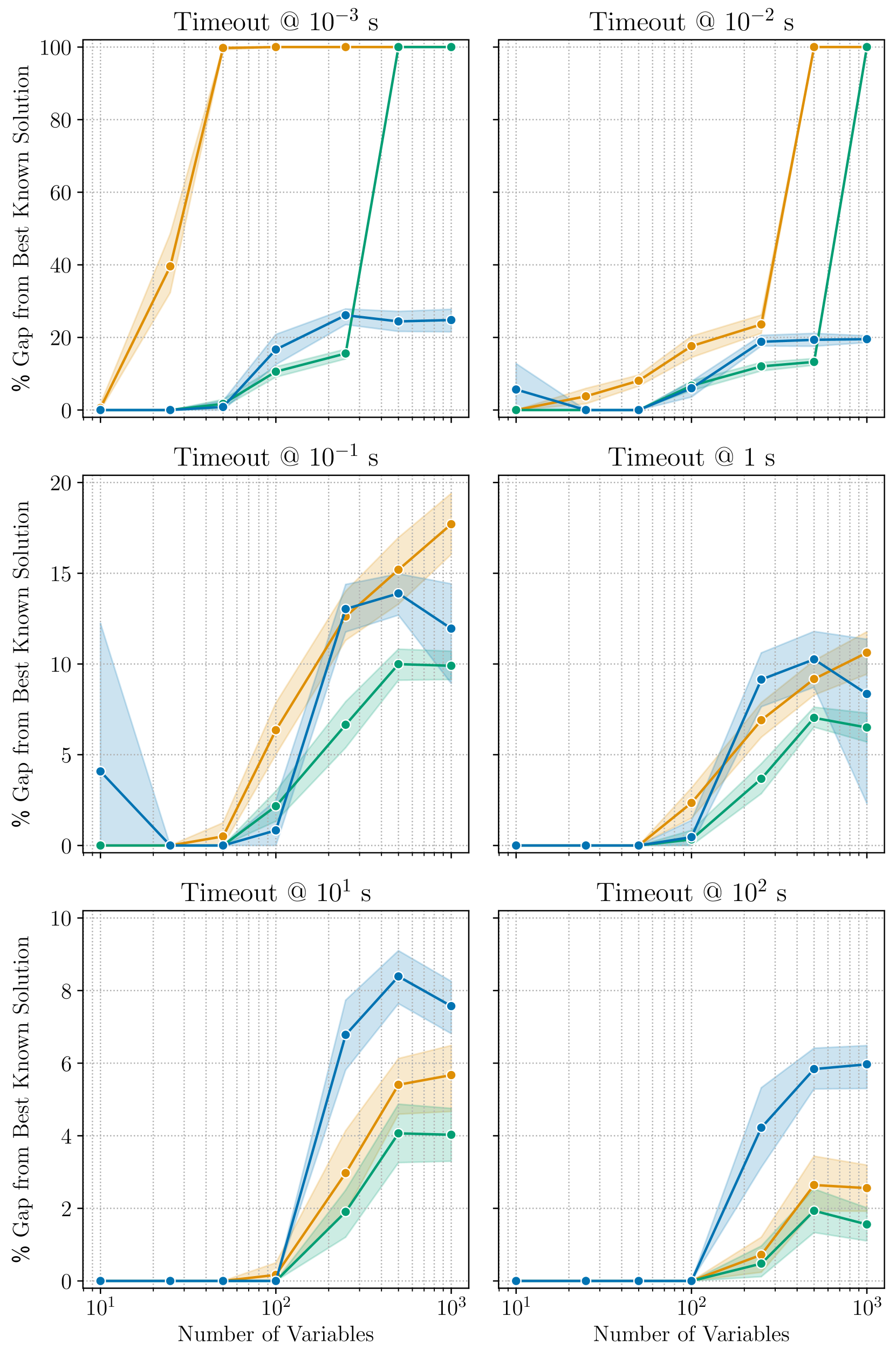
This image presents a 2x3 grid of line plots, each visualizing the performance of different optimization algorithms as a function of the number of variables in the problem, under different timeout constraints. The y-axis represents the "% Gap from Best Known Solution", indicating the suboptimality of the solution found, while the x-axis represents the "Number of Variables" on a logarithmic scale (10<sup>1</sup> to 10<sup>3</sup>). Each plot corresponds to a specific timeout value: 10<sup>-3</sup> s, 10<sup>-2</sup> s, 10<sup>-1</sup> s, 1 s, 10<sup>1</sup> s, and 10<sup>2</sup> s. Each line represents a different algorithm, distinguished by color. Shaded areas around the lines represent the standard deviation or confidence interval.
### Components/Axes
* **X-axis (all plots):** "Number of Variables" (logarithmic scale, from 10<sup>1</sup> to 10<sup>3</sup>).
* **Y-axis (all plots):** "% Gap from Best Known Solution" (linear scale, ranging from 0 to 100 in the top row, 0 to 20 in the middle row, and 0 to 10 in the bottom row).
* **Titles (each plot):** "Timeout @ [Timeout Value] s" (e.g., "Timeout @ 10<sup>-3</sup> s").
* **Lines/Colors:**
* Orange: Algorithm 1
* Blue: Algorithm 2
* Green: Algorithm 3
* Yellow: Algorithm 4
* **Shaded Areas:** Represent the variability (standard deviation or confidence interval) around each line.
### Detailed Analysis
**Plot 1: Timeout @ 10<sup>-3</sup> s (Top-Left)**
* The orange line starts at approximately 40% gap with 10 variables, rises to around 80% with 100 variables, and then decreases slightly to around 60% with 1000 variables.
* The blue line starts at approximately 10% gap, remains relatively stable around 15-20% up to 100 variables, and then increases to around 25% with 1000 variables.
* The green line starts at approximately 20% gap, increases to around 40% with 100 variables, and then decreases to around 30% with 1000 variables.
* The yellow line starts at approximately 20% gap, increases to around 60% with 100 variables, and then decreases to around 40% with 1000 variables.
**Plot 2: Timeout @ 10<sup>-2</sup> s (Top-Right)**
* The orange line starts at approximately 20% gap, increases sharply to around 90% with 100 variables, and then decreases to around 70% with 1000 variables.
* The blue line starts at approximately 5% gap, remains relatively stable around 10-15% up to 100 variables, and then increases to around 20% with 1000 variables.
* The green line starts at approximately 10% gap, increases to around 30% with 100 variables, and then decreases to around 20% with 1000 variables.
* The yellow line starts at approximately 10% gap, increases to around 40% with 100 variables, and then decreases to around 30% with 1000 variables.
**Plot 3: Timeout @ 10<sup>-1</sup> s (Middle-Left)**
* The orange line starts at approximately 5% gap, increases to around 15% with 100 variables, and then remains relatively stable around 10-15% with 1000 variables.
* The blue line starts at approximately 2% gap, remains relatively stable around 5% up to 100 variables, and then increases to around 8% with 1000 variables.
* The green line starts at approximately 5% gap, increases to around 10% with 100 variables, and then remains relatively stable around 8-10% with 1000 variables.
* The yellow line starts at approximately 5% gap, increases to around 12% with 100 variables, and then decreases to around 8% with 1000 variables.
**Plot 4: Timeout @ 1 s (Middle-Right)**
* The orange line starts at approximately 2% gap, increases to around 8% with 100 variables, and then remains relatively stable around 6-8% with 1000 variables.
* The blue line starts at approximately 1% gap, remains relatively stable around 2-3% up to 100 variables, and then increases to around 5% with 1000 variables.
* The green line starts at approximately 2% gap, increases to around 6% with 100 variables, and then remains relatively stable around 5-6% with 1000 variables.
* The yellow line starts at approximately 2% gap, increases to around 7% with 100 variables, and then remains relatively stable around 6-7% with 1000 variables.
**Plot 5: Timeout @ 10<sup>1</sup> s (Bottom-Left)**
* The orange line starts at approximately 1% gap, increases to around 4% with 100 variables, and then remains relatively stable around 3-4% with 1000 variables.
* The blue line starts at approximately 0.5% gap, remains relatively stable around 1-2% up to 100 variables, and then increases to around 3% with 1000 variables.
* The green line starts at approximately 1% gap, increases to around 3% with 100 variables, and then remains relatively stable around 2-3% with 1000 variables.
* The yellow line starts at approximately 1% gap, increases to around 3% with 100 variables, and then remains relatively stable around 2-3% with 1000 variables.
**Plot 6: Timeout @ 10<sup>2</sup> s (Bottom-Right)**
* The orange line starts at approximately 1% gap, increases to around 3% with 100 variables, and then remains relatively stable around 2-3% with 1000 variables.
* The blue line starts at approximately 0.5% gap, remains relatively stable around 1-2% up to 100 variables, and then increases to around 2.5% with 1000 variables.
* The green line starts at approximately 1% gap, increases to around 2.5% with 100 variables, and then remains relatively stable around 2-2.5% with 1000 variables.
* The yellow line starts at approximately 1% gap, increases to around 2.5% with 100 variables, and then remains relatively stable around 2-2.5% with 1000 variables.
### Key Observations
* As the timeout increases, the "% Gap from Best Known Solution" generally decreases for all algorithms. This indicates that longer runtimes allow the algorithms to find better solutions.
* The orange algorithm consistently exhibits the largest gap from the best known solution, especially at shorter timeouts.
* The blue algorithm consistently exhibits the smallest gap from the best known solution across all timeouts.
* The shaded areas indicate that the variability in performance is relatively low, suggesting that the results are consistent.
* The gap tends to plateau or even decrease slightly as the number of variables increases beyond 100, suggesting diminishing returns from increased computation time.
### Interpretation
The data demonstrates the trade-off between computational time and solution quality in optimization algorithms. Increasing the timeout allows the algorithms to explore the solution space more thoroughly, leading to lower gaps from the best-known solution. However, there is a point of diminishing returns, where increasing the timeout further does not significantly improve the solution quality. The blue algorithm appears to be the most efficient, consistently finding solutions closest to the optimum within a given time constraint. The orange algorithm is the least efficient, requiring significantly longer runtimes to achieve comparable performance. The consistent performance of the blue algorithm suggests it may be a more robust or well-suited algorithm for this type of problem. The plots reveal that the problem's difficulty increases with the number of variables, but the algorithms can mitigate this effect with sufficient computational resources (longer timeouts). The consistent trends across the plots suggest a systematic relationship between timeout, problem size, and solution quality, which could be further investigated through statistical modeling.
DECODING INTELLIGENCE...