# Technical Data Extraction: Current Density Streamline Plots
This document provides a detailed technical extraction of the data and visual components from the provided image, which consists of two side-by-side streamline plots representing physical simulations (likely electron transport in a nanostructure).
## 1. General Layout and Metadata
The image contains two subplots, labeled **(a)** and **(c)**. Both plots share the same spatial dimensions and coordinate system.
* **Language:** English
* **Horizontal Axis (x):** `length (nm)`
* **Range:** -50 to 50 nm
* **Markers:** -40, -20, 0, 20, 40
* **Vertical Axis (y):** `width (nm)`
* **Range:** -15 to 15 nm (approximate)
* **Markers:** -10, 0, 10
* **Color Scale (Legend):** Located to the right of each plot. It represents a normalized intensity or magnitude.
* **Color Gradient:** White (0.0) $\rightarrow$ Light Orange $\rightarrow$ Dark Red/Brown (0.6+)
* **Scale Markers:** 0.0, 0.2, 0.4, 0.6
---
## 2. Subplot (a) Analysis
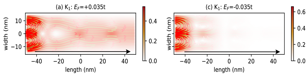
**Header Label:** (a) $K_1: E_F = +0.035t$
### Component Isolation
* **Physical Context:** This plot represents a state with positive Fermi energy ($E_F$).
* **Visual Trend:** The streamlines originate from the left boundary ($x \approx -50$) and propagate toward the right. The intensity (indicated by the red/orange background) is sustained across the entire length of the channel.
* **Flow Pattern:**
* **Injection Point:** High intensity (dark red) at the left boundary, concentrated around $y = \pm 10$ and $y = 0$.
* **Central Region:** The flow exhibits a "braided" or undulating pattern. There are clear nodes of lower intensity (white spots) centered at approximately $x = -35$, $x = -15$, and $x = 25$.
* **Transmission:** The streamlines continue through the right boundary ($x = 50$), indicating high transmission/conductivity.
* **Color/Magnitude Data:**
* Peak values ($\approx 0.5$) are found at the injection site ($x = -50$).
* The intensity remains relatively high (orange hue, $\approx 0.2 - 0.3$) even at the far right of the plot.
---
## 3. Subplot (c) Analysis
**Header Label:** (c) $K_1: E_F = -0.035t$
### Component Isolation
* **Physical Context:** This plot represents a state with negative Fermi energy ($E_F$).
* **Visual Trend:** Unlike subplot (a), the flow in this plot is heavily attenuated. While it starts with high intensity on the left, it fades to near-zero (white) before reaching the center of the channel.
* **Flow Pattern:**
* **Injection Point:** High intensity (dark red) at the left boundary, similar to plot (a).
* **Decay:** The streamlines and the background color intensity drop sharply as $x$ increases.
* **Cut-off:** By $x = 0$, the intensity is nearly 0.0 (white). The streamlines become faint and disappear.
* **Transmission:** There is virtually no flow reaching the right boundary ($x = 50$), indicating a "blocked" or non-conducting state.
* **Color/Magnitude Data:**
* Peak values ($\approx 0.6$) are concentrated at the very edge of the left boundary ($x = -50$).
* The intensity drops below $0.1$ by $x = -20$.
---
## 4. Comparative Summary
| Feature | Subplot (a) | Subplot (c) |
| :--- | :--- | :--- |
| **Fermi Energy ($E_F$)** | $+0.035t$ (Positive) | $-0.035t$ (Negative) |
| **Propagation** | Long-range (Full length) | Short-range (Decays rapidly) |
| **Right Boundary State** | Conducting / Active | Non-conducting / Evanescent |
| **Max Intensity** | $\approx 0.5$ | $\approx 0.6$ (at source only) |
| **Visual Indicators** | Sustained orange/red background | Rapid transition to white background |
**Directional Indicator:** Both plots contain a black arrow at the bottom pointing from left to right, confirming the intended direction of transport or the orientation of the nanostructure.