## Flowchart and Graphs: Problem-Solving Strategies and Performance Metrics
### Overview
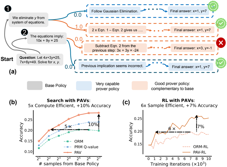
The image contains three components:
1. A flowchart (a) illustrating a problem-solving process for solving a system of equations.
2. Two line graphs (b and c) comparing the performance of different algorithms (ORM, PRM Q-value, PAV) in terms of accuracy and efficiency.
---
### Components/Axes
#### (a) Flowchart
- **Start Node**: "Start" with the question: "Let 4x + 3y = 25, 7x + 6y = 49. Solve for x, y."
- **Step 1**: "We eliminate y from the system of equations."
- **Blue Arrow (0.0)**: Leads to "Follow Gaussian Elimination" → Final answer: x=1, y=7 (✅).
- **Orange Arrow (1.0)**: Leads to "2 × Eqn. 1 – Eqn. 2 gives us..." → Final answer: x=1, y=7 (✅).
- **Step 2**: "The equations imply: 10x + 9y = 25."
- **Blue Arrow (0.0)**: Leads to "Previous implication seems incorrect" → Final answer: x=1, y=7 (✅).
- **Orange Arrow (0.0)**: Leads to "Subtract Eqn. 2 from the previous step: 3x + 3y = -24" → Final answer: x=3, y=-1 (❌).
- **Final Nodes**:
- ✅ Correct answers (x=1, y=7) via Gaussian elimination or 2×Eqn.1–Eqn.2.
- ❌ Incorrect answer (x=3, y=-1) via subtraction.
#### (b) Graph: "Search with PAVs"
- **X-axis**: "# samples from Base Policy" (log scale: 2¹ to 2⁷).
- **Y-axis**: "Accuracy" (0.10 to 0.25).
- **Legend**:
- **ORM** (green dashed line): Starts at ~0.12, peaks at ~0.20.
- **PRM Q-value** (blue dashed line): Starts at ~0.13, peaks at ~0.22.
- **PAV** (orange solid line): Starts at ~0.15, peaks at ~0.25.
- **Annotations**:
- "5× Compute Efficient, +10% Accuracy" (PAV vs. base).
#### (c) Graph: "RL with PAVs"
- **X-axis**: "Training Iterations (×10³)" (0 to 10).
- **Y-axis**: "Accuracy" (0.15 to 0.25).
- **Legend**:
- **ORM-RL** (red dashed line): Starts at ~0.15, peaks at ~0.20.
- **PAV-RL** (orange solid line): Starts at ~0.15, peaks at ~0.25.
- **Annotations**:
- "6× Sample Efficient, +7% Accuracy" (PAV-RL vs. base).
---
### Detailed Analysis
#### (a) Flowchart
- **Flow**:
1. Start → Step 1 (eliminate y).
2. Step 1 branches into two paths:
- Blue (correct): Follows Gaussian elimination → x=1, y=7.
- Orange (incorrect): Subtracts equations → x=3, y=-1.
3. Step 2 branches into two paths:
- Blue (correct): Rejects flawed implication → x=1, y=7.
- Orange (incorrect): Subtracts equations → x=3, y=-1.
#### (b) Graph: "Search with PAVs"
- **Trends**:
- All methods improve accuracy with more samples.
- **PAV** consistently outperforms ORM and PRM Q-value.
- At 2⁷ samples, PAV reaches ~0.25 accuracy (vs. ~0.22 for PRM Q-value and ~0.20 for ORM).
#### (c) Graph: "RL with PAVs"
- **Trends**:
- **PAV-RL** achieves higher accuracy (~0.25) than ORM-RL (~0.20) after 10³ iterations.
- PAV-RL shows sharper improvement (6× sample efficiency).
---
### Key Observations
1. **Flowchart**:
- Gaussian elimination and 2×Eqn.1–Eqn.2 yield correct results.
- Subtracting equations leads to errors.
2. **Graphs**:
- **PAV** methods (search and RL) outperform ORM and PRM Q-value in both accuracy and efficiency.
- PAV-RL achieves 7% higher accuracy than ORM-RL with fewer samples.
---
### Interpretation
- The flowchart demonstrates that **Gaussian elimination** is a reliable method for solving systems of equations, while flawed algebraic manipulations (e.g., subtraction) lead to errors.
- The graphs highlight the **superiority of PAV-based algorithms** in both search and reinforcement learning contexts. PAV methods achieve higher accuracy with fewer computational resources, suggesting they are more efficient and robust for this task.
- The 10% and 7% efficiency gains (PAV vs. base) indicate that PAV reduces the number of samples or iterations needed to reach optimal performance, making it a promising approach for optimization problems.
- The incorrect answer (x=3, y=-1) in the flowchart underscores the importance of method selection in problem-solving, as minor errors in algebraic steps can propagate to wrong conclusions.