## Scatter Plot with Heatmaps and Network Diagram: Normalized Energy vs. I₀ and City Visit Orders
### Overview
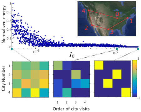
The image combines three primary components:
1. A **scatter plot** showing normalized energy vs. I₀ (logarithmic scale).
2. Three **heatmaps** representing city visit order correlations.
3. A **network diagram** of U.S. cities labeled 0–4.
### Components/Axes
#### Scatter Plot
- **X-axis**: I₀ (logarithmic scale, 10⁻¹ to 10¹).
- **Y-axis**: Normalized energy (0 to 1).
- **Data points**: Blue dots with a power-law decay trend.
- **Inset**: Zoomed-in region highlighting I₀ ≈ 10⁰.
#### Heatmaps
- **X-axis**: Order of city visits (1–4).
- **Y-axis**: City Number (1–4).
- **Color scale**: Green (low) to yellow (high), with a legend ranging from -1 to 1.
- **Heatmaps**:
- **I₀ = 10⁻¹**: Mixed green/yellow (moderate values).
- **I₀ = 10⁰**: Blue/green dominance (lower values).
- **I₀ = 10¹**: Blue/yellow squares (localized high values).
#### Network Diagram
- **Nodes**: Labeled 0–4, connected by red lines.
- **Geographic context**: Map of the U.S. with cities positioned as nodes.
### Detailed Analysis
#### Scatter Plot
- **Trend**: Normalized energy decreases sharply for I₀ < 10⁰, then plateaus.
- **Key data points**:
- At I₀ = 10⁻¹: Energy ≈ 0.8–0.9.
- At I₀ = 10⁰: Energy ≈ 0.2–0.4.
- At I₀ = 10¹: Energy ≈ 0.0–0.1.
#### Heatmaps
- **I₀ = 10⁻¹**:
- City 1: High values (yellow) for visits 1 and 4.
- City 4: High values (yellow) for visits 1 and 3.
- **I₀ = 10⁰**:
- City 2: Moderate values (green) for visits 2 and 3.
- City 3: Low values (blue) for visits 1 and 4.
- **I₀ = 10¹**:
- City 1: High values (yellow) for visits 1 and 4.
- City 4: High values (yellow) for visits 1 and 3.
#### Network Diagram
- **Connections**:
- 0 ↔ 1 ↔ 2 ↔ 3 ↔ 4 (linear chain).
- Additional diagonal links: 0 ↔ 3 and 1 ↔ 4.
### Key Observations
1. **Power-law decay**: Normalized energy drops rapidly for I₀ < 10⁰, then stabilizes.
2. **Heatmap anomalies**:
- At I₀ = 10¹, yellow squares (high values) appear in specific city-visit pairs (e.g., City 1, Visit 1).
- These may indicate localized interactions or feedback loops.
3. **Network structure**: The U.S. city network forms a connected graph with redundant paths (e.g., 0–3 and 1–4 links).
### Interpretation
- **Energy-I₀ relationship**: The power-law decay suggests that energy dissipation is highly sensitive to I₀ at low values but becomes less dependent at higher I₀.
- **Heatmap correlations**: High-energy values (yellow) at I₀ = 10¹ imply that certain city visit orders (e.g., 1→4) amplify energy contributions, possibly due to network topology.
- **Network implications**: The redundant connections (e.g., 0–3 and 1–4) may facilitate energy redistribution, explaining the plateau in the scatter plot.
- **Anomalies**: The localized yellow squares in the I₀ = 10¹ heatmap suggest specific city pairs (e.g., City 1 and 4) have disproportionate influence, warranting further investigation into their physical or systemic properties.
### Spatial Grounding
- **Legend**: Right-aligned for heatmaps, matching color gradients to values.
- **Inset**: Positioned near the lower-left of the scatter plot, focusing on I₀ ≈ 10⁰.
- **Network diagram**: Top-right corner, spatially isolated from heatmaps but thematically linked via city labels.
### Conclusion
The data demonstrates a strong interplay between I₀, city visit order, and network structure in determining normalized energy. The anomalies in the heatmaps highlight the need to explore localized interactions within the network, potentially revealing hidden dependencies or feedback mechanisms.