## Diagram: Instruction Sequence and DAG Representation
### Overview
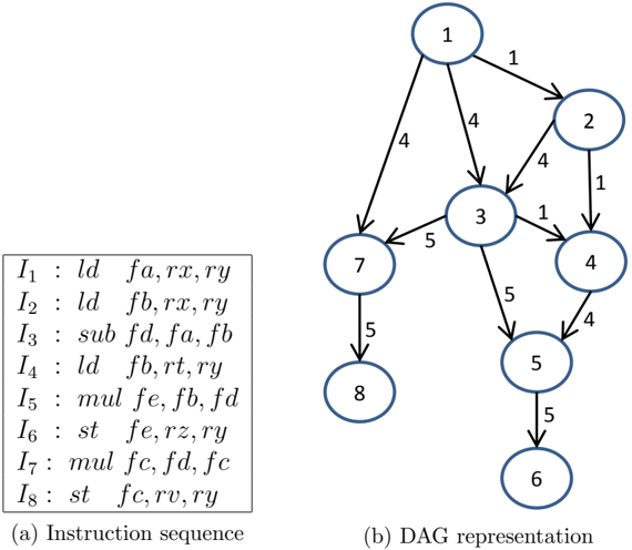
The image presents two distinct but related components:
1. **Left:** A textual list of assembly-style instructions labeled $I_1$ through $I_8$.
2. **Right:** A Directed Acyclic Graph (DAG) labeled (b), which visually maps the dependencies and execution flow of the instructions listed on the left.
### Components/Axes
#### (a) Instruction Sequence
This is a vertical list of 8 instructions, formatted as `Label : Operation Destination, Source1, Source2`.
* $I_1 : ld \quad fa, rx, ry$
* $I_2 : ld \quad fb, rx, ry$
* $I_3 : sub \quad fd, fa, fb$
* $I_4 : ld \quad fb, rt, ry$
* $I_5 : mul \quad fe, fb, fd$
* $I_6 : st \quad fe, rz, ry$
* $I_7 : mul \quad fc, fd, fc$
* $I_8 : st \quad fc, rv, ry$
#### (b) DAG Representation
This is a directed graph consisting of 8 nodes (numbered 1 through 8) and 11 directed edges. Each edge is labeled with a numerical weight, likely representing instruction latency or dependency distance.
* **Nodes:** Represent the instructions $I_1$ through $I_8$.
* **Edges:** Represent the flow of data or control dependency between instructions.
* **Weights:** Numerical values (1, 4, 5) assigned to each edge.
### Detailed Analysis
#### Instruction Sequence Breakdown
The instructions appear to be a sequence of memory loads (`ld`), arithmetic operations (`sub`, `mul`), and memory stores (`st`).
* **Loads:** $I_1, I_2, I_4$
* **Arithmetic:** $I_3$ (subtraction), $I_5$ (multiplication), $I_7$ (multiplication)
* **Stores:** $I_6, I_8$
#### DAG Structure and Connectivity
The graph is organized with Node 1 at the top (root) and Nodes 6 and 8 at the bottom (sinks).
| Source Node | Destination Node | Weight |
| :--- | :--- | :--- |
| 1 | 2 | 1 |
| 1 | 3 | 4 |
| 1 | 7 | 4 |
| 2 | 3 | 4 |
| 2 | 4 | 1 |
| 3 | 4 | 1 |
| 3 | 5 | 5 |
| 3 | 7 | 5 |
| 4 | 5 | 4 |
| 5 | 6 | 5 |
| 7 | 8 | 5 |
### Key Observations
* **Root Node:** Node 1 is the sole entry point, branching out to nodes 2, 3, and 7.
* **Sink Nodes:** The graph terminates at Node 6 and Node 8.
* **Parallelism:** The graph shows distinct parallel paths. One path flows through $1 \rightarrow 7 \rightarrow 8$, while another flows through $1 \rightarrow 2 \rightarrow 4 \rightarrow 5 \rightarrow 6$.
* **High-Latency Edges:** The edges with weight 5 (e.g., $3 \rightarrow 5$, $3 \rightarrow 7$, $5 \rightarrow 6$, $7 \rightarrow 8$) represent the longest dependency chains or highest latency operations in the sequence.
* **Convergence:** Node 3 acts as a significant hub, receiving inputs from 1 and 2, and distributing to 4, 5, and 7.
### Interpretation
This diagram is a standard representation used in compiler design and computer architecture to visualize **Data Dependency Graphs**.
* **Instruction Mapping:** The nodes 1-8 correspond directly to the instructions $I_1-I_8$.
* **Dependency Logic:** The edges represent "Read-After-Write" (RAW) or similar data dependencies. For example, $I_3$ (Node 3) requires the results of $I_1$ and $I_2$ (Nodes 1 and 2), which is reflected by the incoming edges from 1 and 2 to 3.
* **Optimization Insight:** The DAG allows a compiler or processor to identify which instructions can be executed in parallel. For instance, the path $1 \rightarrow 7 \rightarrow 8$ is largely independent of the path $2 \rightarrow 4 \rightarrow 5 \rightarrow 6$ after the initial branching from Node 1.
* **Latency Modeling:** The weights on the edges (1, 4, 5) likely correspond to the number of clock cycles required for the result of the source instruction to be available for the destination instruction. The "5" weight edges suggest critical paths that determine the overall execution time of the instruction block.