## Directed Acyclic Graph (DAG) Diagram: Instruction Dependency and Latency
### Overview
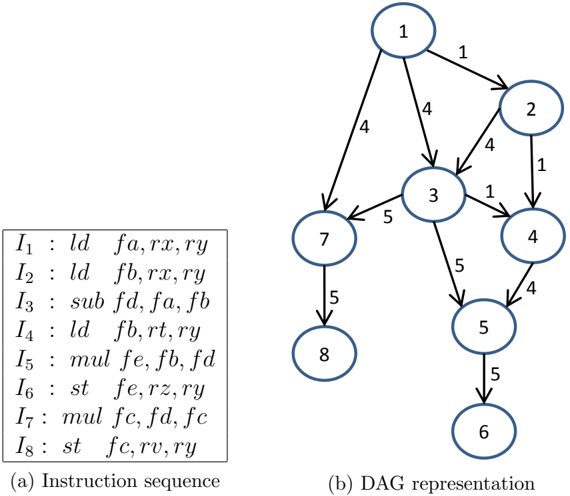
The image presents a technical diagram consisting of two interconnected components: a sequence of assembly-like instructions and a corresponding Directed Acyclic Graph (DAG) that models the data dependencies and operation latencies between those instructions. The diagram is used to visualize instruction-level parallelism and scheduling in a processor or compiler context.
### Components/Axes
The image is divided into two labeled sections:
1. **(a) Instruction sequence**: A text box on the left containing eight instructions, labeled `I₁` through `I₈`.
2. **(b) DAG representation**: A graph on the right with eight circular nodes (numbered 1-8) connected by directed edges. Each edge has a numerical weight.
**Instruction Sequence (a):**
The instructions are listed as follows:
* `I₁ : ld fa, rx, ry`
* `I₂ : ld fb, rx, ry`
* `I₃ : sub fd, fa, fb`
* `I₄ : ld fb, rt, ry`
* `I₅ : mul fe, fb, fd`
* `I₆ : st fe, rz, ry`
* `I₇ : mul fc, fd, fc`
* `I₈ : st fc, rv, ry`
**DAG Representation (b):**
* **Nodes**: Eight nodes, numbered 1 through 8, correspond directly to instructions `I₁` through `I₈`.
* **Edges & Weights**: Directed edges connect nodes, with arrows indicating the direction of data dependency. A number on each edge represents a weight, likely indicating the latency (in cycles) of the source operation.
* Node 1 → Node 2 (weight: 1)
* Node 1 → Node 3 (weight: 4)
* Node 1 → Node 7 (weight: 4)
* Node 2 → Node 3 (weight: 4)
* Node 2 → Node 4 (weight: 1)
* Node 3 → Node 4 (weight: 1)
* Node 3 → Node 5 (weight: 5)
* Node 3 → Node 7 (weight: 5)
* Node 4 → Node 5 (weight: 4)
* Node 5 → Node 6 (weight: 5)
* Node 7 → Node 8 (weight: 5)
### Detailed Analysis
**Instruction-to-Node Mapping:**
* `I₁` (Load `fa`) = Node 1
* `I₂` (Load `fb`) = Node 2
* `I₃` (Subtract `fd = fa - fb`) = Node 3
* `I₄` (Load `fb` again) = Node 4
* `I₅` (Multiply `fe = fb * fd`) = Node 5
* `I₆` (Store `fe`) = Node 6
* `I₇` (Multiply `fc = fd * fc`) = Node 7
* `I₈` (Store `fc`) = Node 8
**Dependency Flow & Latency Analysis:**
The DAG reveals the critical path and parallel execution opportunities.
1. **Initial Loads**: Nodes 1 and 2 (`I₁`, `I₂`) are independent roots. They have a latency of 1 cycle each (edge to nodes 2 and 4).
2. **First Computation**: Node 3 (`I₃`, subtract) depends on the results from both Node 1 and Node 2. The edges from 1→3 and 2→3 both have a weight of 4, indicating the `ld` operations have a 4-cycle latency before their results are available for the `sub`.
3. **Second Load & Further Computation**: Node 4 (`I₄`, another load of `fb`) depends on Node 2 (weight 1) and Node 3 (weight 1). Node 5 (`I₅`, multiply) depends on Node 3 (weight 5) and Node 4 (weight 4). This shows the result of the subtract (`fd`) and the new load (`fb`) are both needed for the multiply.
4. **Store Operations**: Node 6 (`I₆`) depends solely on Node 5 (weight 5). Node 8 (`I₈`) depends solely on Node 7 (weight 5).
5. **Parallel Branch**: Node 7 (`I₇`, another multiply) has two dependencies: from Node 1 (weight 4) and Node 3 (weight 5). This creates a parallel computation path alongside the path through Node 5.
**Latency Pattern Inference:**
Based on the edge weights, the approximate operation latencies are:
* `ld` (Load): 1 cycle (edge from load to next dependent).
* `sub` (Subtract): 4 cycles.
* `mul` (Multiply): 5 cycles.
* `st` (Store): 5 cycles.
### Key Observations
1. **Register Reuse and Overwrite**: Register `fb` is loaded twice (`I₂` and `I₄`). The DAG correctly models this by having Node 4 depend on the earlier Node 2, not on the original `fb` value from Node 2 for its own operation.
2. **Critical Path**: The longest dependency chain appears to be: Node 1 → Node 3 → Node 5 → Node 6. Summing the edge weights (4 + 5 + 5) gives a minimum latency of 14 cycles for this path.
3. **Parallelism**: The graph shows two main branches after Node 3: one leading to Node 5/6 and another leading to Node 7/8. These can execute in parallel once the dependencies from Node 1 and Node 3 are satisfied.
4. **Anti-dependency**: The sequence shows a Write-After-Read (WAR) anti-dependency on register `fb` between `I₂` and `I₄`. The DAG handles this by treating `I₄` as a new load, dependent on the prior instruction that used `fb` (`I₂`).
### Interpretation
This diagram is a fundamental tool in computer architecture and compiler design for **instruction scheduling**. It visually answers: "Which instructions must wait for others, and how long must they wait?"
* **What it demonstrates**: The DAG explicitly maps data flow dependencies. An instruction (node) can only execute once all its predecessor nodes have completed and their results are available after the specified latency. The weights quantify the waiting time.
* **How elements relate**: The instruction sequence (a) is the source code. The DAG (b) is its dependency graph, abstracting away syntax to focus on data flow and timing. The node numbers provide a direct cross-reference.
* **Notable patterns**: The graph highlights that while the instruction sequence is linear, the underlying operations have significant parallel potential (the two `mul` branches). A smart scheduler could interleave instructions from the two branches to hide latency and improve performance.
* **Underlying purpose**: This model is used to build a **schedule**—a reordered sequence of instructions that respects dependencies while minimizing total execution time (the critical path length). The goal is to keep the processor's functional units busy by issuing independent instructions concurrently.