## Chart/Diagram Type: Multi-Panel Figure: Programming of ReRAM
### Overview
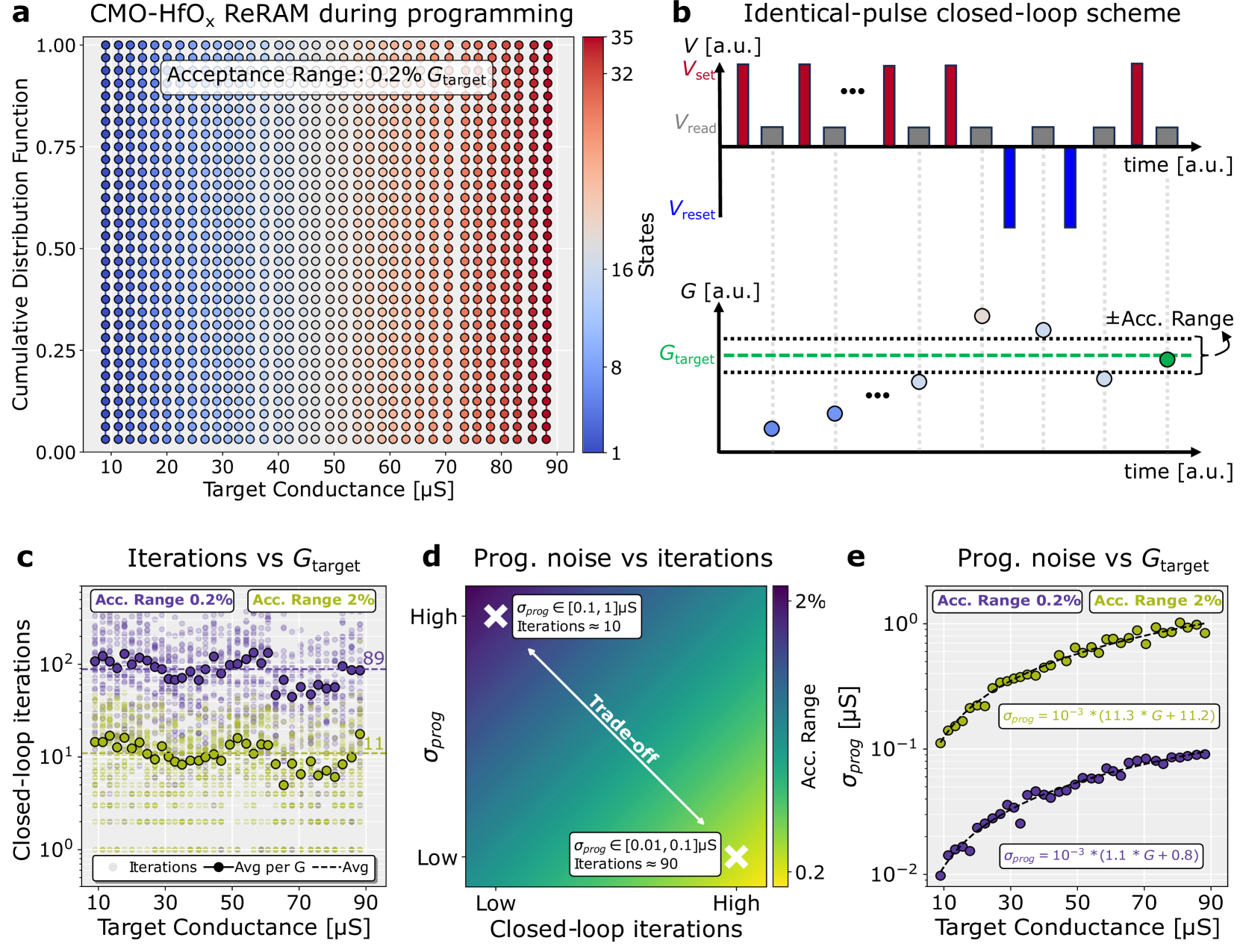
The image presents a multi-panel figure (a-e) illustrating the programming of a CMO-HfOₓ ReRAM (Resistive Random-Access Memory) using a closed-loop scheme. The figure explores the relationship between target conductance, programming noise, and the number of iterations required for programming.
### Components/Axes
**Panel a: Cumulative Distribution Function vs. Target Conductance**
* **Title:** CMO-HfOₓ ReRAM during programming
* **Axes:**
* X-axis: Target Conductance [µS], ranging from 10 to 90 in increments of 10.
* Y-axis: Cumulative Distribution Function, ranging from 0.00 to 1.00 in increments of 0.25.
* **Color Scale:** A color gradient from blue to red, representing the number of states, ranging from 1 to 35.
* **Annotation:** "Acceptance Range: 0.2% Gtarget"
**Panel b: Identical-pulse closed-loop scheme**
* **Title:** Identical-pulse closed-loop scheme
* **Top Subplot Axes:**
* Y-axis: V [a.u.] (Arbitrary Units)
* Annotations: Vset (red), Vread (gray), Vreset (blue)
* X-axis: time [a.u.] (Arbitrary Units)
* **Bottom Subplot Axes:**
* Y-axis: G [a.u.] (Arbitrary Units)
* Annotation: Gtarget (green, dashed line)
* X-axis: time [a.u.] (Arbitrary Units)
* Annotation: ±Acc. Range (green bracket)
**Panel c: Iterations vs Gtarget**
* **Title:** Iterations vs Gtarget
* **Axes:**
* X-axis: Target Conductance [µS], ranging from 10 to 90 in increments of 20.
* Y-axis: Closed-loop iterations (logarithmic scale), ranging from 10⁰ to 10².
* **Data Series:**
* Iterations (gray dots)
* Avg per G (yellow dots)
* Avg (dashed lines):
* Acceptance Range 0.2% (purple, average around 89 iterations)
* Acceptance Range 2% (yellow, average around 11 iterations)
* **Annotations:** "Acc. Range 0.2%", "Acc. Range 2%"
**Panel d: Prog. noise vs iterations**
* **Title:** Prog. noise vs iterations
* **Axes:**
* X-axis: Closed-loop iterations (qualitative, Low to High)
* Y-axis: σprog (qualitative, Low to High)
* **Color Scale:** A color gradient from purple to yellow, representing the Acceptance Range, ranging from 0.2% to 2%.
* **Annotations:**
* "Trade-off" (white arrow)
* "σprog ∈ [0.1, 1] µS, Iterations ≈ 10" (white cross at top-left)
* "σprog ∈ [0.01, 0.1] µS, Iterations ≈ 90" (white cross at bottom-right)
**Panel e: Prog. noise vs Gtarget**
* **Title:** Prog. noise vs Gtarget
* **Axes:**
* X-axis: Target Conductance [µS], ranging from 10 to 90 in increments of 20.
* Y-axis: σprog [µS] (logarithmic scale), ranging from 10⁻² to 10⁰.
* **Data Series:**
* Acceptance Range 0.2% (purple dots): σprog = 10⁻³ * (1.1 * G + 0.8)
* Acceptance Range 2% (yellow dots): σprog = 10⁻³ * (11.3 * G + 11.2)
* **Annotations:** "Acc. Range 0.2%", "Acc. Range 2%"
### Detailed Analysis
**Panel a:** The cumulative distribution function shows how the states are distributed across different target conductance values. The color gradient indicates the density of states, with blue representing lower states and red representing higher states. The distribution shifts towards higher conductance values as the target conductance increases.
**Panel b:** This panel illustrates the identical-pulse closed-loop scheme. The top subplot shows the voltage pulses applied (Vset, Vread, Vreset) over time. The bottom subplot shows the resulting conductance (G) over time, converging towards the target conductance (Gtarget) within an acceptable range (±Acc. Range).
**Panel c:** This graph shows the relationship between the number of closed-loop iterations and the target conductance. The gray dots represent individual iterations, while the yellow dots represent the average number of iterations for each target conductance. The dashed lines indicate the average number of iterations for acceptance ranges of 0.2% (purple, ~89 iterations) and 2% (yellow, ~11 iterations).
**Panel d:** This heatmap illustrates the trade-off between programming noise (σprog) and the number of closed-loop iterations. Lower noise requires more iterations, and vice versa. The color gradient represents the acceptance range, with purple indicating a tighter acceptance range (0.2%) and yellow indicating a wider acceptance range (2%).
**Panel e:** This graph shows the relationship between programming noise (σprog) and target conductance. The purple dots represent an acceptance range of 0.2%, and the yellow dots represent an acceptance range of 2%. The equations provided describe the relationship between σprog and G for each acceptance range.
### Key Observations
* **Panel a:** The distribution of states shifts towards higher conductance values as the target conductance increases.
* **Panel b:** The closed-loop scheme converges towards the target conductance over time.
* **Panel c:** A tighter acceptance range (0.2%) requires significantly more iterations than a wider acceptance range (2%).
* **Panel d:** There is a clear trade-off between programming noise and the number of iterations.
* **Panel e:** Programming noise increases with target conductance for both acceptance ranges.
### Interpretation
The data presented in this figure demonstrates the programming characteristics of a CMO-HfOₓ ReRAM using a closed-loop scheme. The key findings are:
1. **Trade-off between Accuracy and Speed:** A tighter acceptance range (higher accuracy) requires more programming iterations (slower programming).
2. **Programming Noise Increases with Target Conductance:** As the target conductance increases, the programming noise also increases, making it more challenging to achieve precise programming at higher conductance levels.
3. **Closed-Loop Scheme Effectiveness:** The closed-loop scheme effectively converges towards the target conductance, but the number of iterations required depends on the desired accuracy and the target conductance value.
The figure highlights the importance of carefully considering the trade-offs between accuracy, speed, and noise when programming ReRAM devices. The data can be used to optimize programming algorithms and device parameters to achieve the desired performance characteristics.