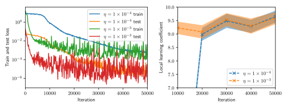
## Line Graphs: Training and Test Loss vs. Local Learning Coefficient ### Overview The image contains two line graphs. The left graph shows training and test loss over iterations for different learning rates (η). The right graph displays the local learning coefficient over iterations for the same learning rates. Both graphs use logarithmic and linear scales, respectively, with shaded regions indicating variability or confidence intervals. --- ### Components/Axes #### Left Graph (Train and Test Loss) - **X-axis**: "Iteration" (0 to 50,000, linear scale). - **Y-axis**: "Train and test loss" (logarithmic scale: 10⁻⁶ to 10⁰). - **Legend**: - Blue line: η = 1 × 10⁻⁴ (train). - Orange line: η = 1 × 10⁻⁴ (test). - Green line: η = 1 × 10⁻³ (train). - Red line: η = 1 × 10⁻³ (test). #### Right Graph (Local Learning Coefficient) - **X-axis**: "Iteration" (0 to 50,000, linear scale). - **Y-axis**: "Local learning coefficient" (linear scale: 7.0 to 10.0). - **Legend**: - Blue line with crosses: η = 1 × 10⁻⁴. - Orange line with crosses: η = 1 × 10⁻³. - **Shaded regions**: Confidence intervals (light orange for η = 1 × 10⁻³). --- ### Detailed Analysis #### Left Graph 1. **Blue line (η = 1 × 10⁻⁴, train)**: - Starts at ~10⁰, decreases smoothly to ~10⁻⁴ by iteration 50,000. - Minimal fluctuations after initial drop. 2. **Orange line (η = 1 × 10⁻⁴, test)**: - Starts at ~10⁻¹, decreases to ~10⁻³ by iteration 50,000. - Slight oscillations but generally stable. 3. **Green line (η = 1 × 10⁻³, train)**: - Starts at ~10⁻², decreases to ~10⁻⁴ by iteration 50,000. - More volatility than blue line, especially early on. 4. **Red line (η = 1 × 10⁻³, test)**: - Starts at ~10⁻³, fluctuates between 10⁻⁴ and 10⁻⁵. - Highest volatility, ending near 10⁻⁵. #### Right Graph 1. **Blue line (η = 1 × 10⁻⁴)**: - Starts at 9.5, drops sharply to 8.5 by iteration 20,000. - Rises to 9.0 by iteration 50,000. - Shaded region (confidence interval) narrows after 20,000. 2. **Orange line (η = 1 × 10⁻³)**: - Starts at 9.0, dips to 8.0 by iteration 20,000. - Rises to 9.5 by iteration 50,000. - Wider shaded region indicates higher variability. --- ### Key Observations 1. **Left Graph**: - Smaller η (1 × 10⁻⁴) results in smoother convergence for both train and test loss. - Larger η (1 × 10⁻³) exhibits higher volatility, especially in test loss. - Test loss consistently lags behind train loss for both η values. 2. **Right Graph**: - η = 1 × 10⁻⁴ shows a sharp initial drop in local learning coefficient, stabilizing afterward. - η = 1 × 10⁻³ has more pronounced fluctuations but ends at a higher value (9.5 vs. 9.0). - Confidence intervals for η = 1 × 10⁻³ are broader, suggesting less certainty in its trajectory. --- ### Interpretation - **Learning Rate Impact**: - Smaller η (1 × 10⁻⁴) ensures stability in both loss and local learning coefficient, albeit with slower initial progress. - Larger η (1 × 10⁻³) accelerates early changes but introduces instability, risking suboptimal convergence. - **Trade-offs**: - The local learning coefficient for η = 1 × 10⁻³ ends higher, suggesting potential for better performance despite volatility. - The sharp drop in η = 1 × 10⁻⁴’s local learning coefficient may indicate an initial adjustment phase before stabilization. - **Anomalies**: - The red line (η = 1 × 10⁻³, test) in the left graph shows erratic behavior, possibly due to overfitting or sensitivity to noise. - The right graph’s shaded regions highlight that η = 1 × 10⁻³’s local learning coefficient is less predictable. This analysis underscores the balance between learning rate magnitude and model stability, with smaller rates favoring consistency and larger rates offering potential gains at the cost of variability.