\n
## Diagram: Attention Mechanism in Sequence-to-Sequence Model
### Overview
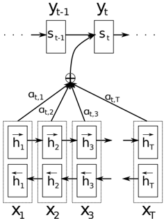
The image is a technical diagram illustrating the architecture of an attention mechanism within a sequence-to-sequence (seq2seq) model, likely for tasks like machine translation or time series prediction. It visually represents how the model's decoder at a given time step `t` focuses on different parts of the input sequence by computing attention weights.
### Components/Axes
The diagram is structured into three main horizontal layers, showing the flow of information from bottom to top.
**1. Bottom Layer (Input Sequence Encoder):**
* **Elements:** A series of rectangular blocks representing the encoder's hidden states for an input sequence of length `T`.
* **Labels (from left to right):**
* `x₁`, `x₂`, `x₃`, ..., `x_T`: These are the input elements (e.g., words, time steps).
* Inside each block, there are two sub-components:
* `h→₁`, `h→₂`, `h→₃`, ..., `h→_T`: The forward hidden states.
* `h←₁`, `h←₂`, `h←₃`, ..., `h←_T`: The backward hidden states.
* **Flow:** Arrows indicate the bidirectional processing. The forward states (`h→`) are connected left-to-right, and the backward states (`h←`) are connected right-to-left. This indicates a **Bidirectional Recurrent Neural Network (BiRNN)** encoder.
**2. Middle Layer (Attention Mechanism):**
* **Elements:** A central summation node (denoted by `⊕`) and connecting lines with labels.
* **Labels:**
* `α_{t,1}`, `α_{t,2}`, `α_{t,3}`, ..., `α_{t,T}`: These are the **attention weights** (or alignment scores). They are scalars associated with each encoder hidden state `h_i` for the current decoder time step `t`.
* **Flow:** Lines connect each encoder hidden state (the combined forward/backward representation) to the summation node. The labels `α_{t,i}` are placed on these lines, indicating that each hidden state is weighted by its corresponding attention coefficient before being summed.
**3. Top Layer (Decoder State):**
* **Elements:** A sequence of rectangular blocks representing the decoder's hidden states over time.
* **Labels (from left to right):**
* `s_{t-1}`: The decoder's hidden state from the previous time step.
* `s_t`: The decoder's hidden state for the current time step `t`.
* `y_{t-1}`, `y_t`: The output predictions (e.g., generated words) corresponding to the decoder states.
* **Flow:** An arrow points from `s_{t-1}` to `s_t`, showing the recurrent connection. A curved arrow originates from the summation node (`⊕`) and points into the `s_t` block. This is the **context vector**, which is the weighted sum of encoder states and serves as a key input for generating the new decoder state `s_t`.
### Detailed Analysis
* **Process Flow:** The diagram depicts a single computational step at decoder time `t`.
1. The decoder's previous state `s_{t-1}` is used to compute attention scores against all encoder hidden states (`h_i`).
2. These scores are normalized (likely via a softmax function, not shown) to produce the attention weights `α_{t,1}` through `α_{t,T}`. The sum of all `α_{t,i}` for a given `t` should equal 1.
3. The encoder hidden states are combined into a single **context vector** via a weighted sum: `Context_t = Σ_{i=1 to T} (α_{t,i} * h_i)`. This is represented by the `⊕` node.
4. This context vector, along with `s_{t-1}` and possibly the previous output `y_{t-1}`, is used to compute the new decoder state `s_t`.
5. The state `s_t` is then used to generate the output `y_t`.
* **Spatial Grounding:** The legend (the attention weights `α_{t,i}`) is not in a separate box but is integrated directly onto the connecting lines in the middle of the diagram. The placement of `α_{t,1}` on the leftmost line and `α_{t,T}` on the rightmost line corresponds directly to the first (`x₁`) and last (`x_T`) input elements.
### Key Observations
1. **Bidirectional Encoding:** The presence of both `h→` and `h←` confirms the use of a BiRNN, which captures context from both past and future in the input sequence.
2. **Dynamic Context:** The context vector for decoder step `t` is not fixed; it is dynamically computed based on `s_{t-1}`. This allows the model to "attend" to different parts of the input sequence at each output step.
3. **Temporal Unfolding:** The diagram shows a "slice" of the process at time `t`. The ellipses (`...`) on the left and right of the encoder and decoder sequences indicate that this is part of a longer sequence.
4. **Information Bottleneck:** The architecture shows how a variable-length input sequence (`x₁...x_T`) is compressed into a fixed-dimensional context vector at each step, which is then used by the decoder.
### Interpretation
This diagram is a canonical representation of the **Bahdanau et al. (2014) style attention mechanism**. It solves a fundamental limitation of the original seq2seq model, where the entire input sequence was compressed into a single, fixed-length context vector (the final encoder state), creating an information bottleneck for long sequences.
The key insight visualized here is that the decoder should have **direct, selective access to the entire input sequence**. The attention weights `α_{t,i}` act as a "soft alignment" between the decoder's current focus (represented by `s_{t-1}`) and each part of the input. For example, in translation, when generating the t-th word in the target sentence, the model can learn to place high attention weight `α_{t,i}` on the i-th word in the source sentence that is most relevant.
The diagram emphasizes the **interdependency** of the components: the decoder state `s_t` depends on the context vector, which in turn depends on all encoder states and the attention weights, which are themselves computed from the previous decoder state `s_{t-1}`. This creates a powerful, differentiable mechanism for learning what to focus on within sequential data.