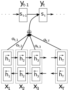
## Diagram: Hidden Markov Model (HMM) Structure ### Overview The diagram illustrates a Hidden Markov Model (HMM) framework, depicting state transitions, hidden states, and observations over time. It includes temporal dependencies (Y_{t-1}, Y_t), hidden states (h₁, h₂, h₃, h_T), observations (X₁, X₂, X₃, X_T), and transition probabilities (α_{t,1}, α_{t,2}, α_{t,3}, α_{t,T}). ### Components/Axes 1. **Top Section (State Transitions):** - **Labels:** Y_{t-1}, Y_t, S_{t-1}, S_t. - **Flow:** Arrows indicate sequential transitions from S_{t-1} → S_t, with Y_{t-1} and Y_t as outputs. - **Positioning:** Y_{t-1} and Y_t are positioned above S_{t-1} and S_t, respectively. 2. **Bottom Section (Hidden States and Observations):** - **Hidden States:** h₁, h₂, h₃, h_T (represented as vertical boxes with bidirectional arrows). - **Observations:** X₁, X₂, X₃, X_T (labeled below hidden states). - **Transition Probabilities:** α_{t,1}, α_{t,2}, α_{t,3}, α_{t,T} (labeled as diagonal arrows connecting S_t to hidden states and observations). 3. **Central Node:** - A summation node (⊕) connects S_t to the hidden states and observations, suggesting aggregation or combination of states. ### Detailed Analysis - **State Transitions (Top):** - S_{t-1} transitions to S_t, with Y_{t-1} and Y_t as outputs. This implies a Markovian process where the current state (S_t) depends only on the previous state (S_{t-1}). - **Hidden States and Observations (Bottom):** - Hidden states (h₁, h₂, h₃, h_T) are interconnected with bidirectional arrows, indicating possible transitions between them. - Observations (X₁, X₂, X₃, X_T) are linked to hidden states via bidirectional arrows, suggesting that each hidden state emits an observation. - Transition probabilities (α_{t,1}, α_{t,2}, α_{t,3}, α_{t,T}) quantify the likelihood of transitioning from S_t to each hidden state or observation. - **Spatial Relationships:** - The top section (state transitions) is spatially separated from the bottom section (hidden states/observations), emphasizing distinct layers of the model. - The central summation node (⊕) acts as a bridge between S_t and the hidden states/observations. ### Key Observations 1. **Temporal Structure:** The diagram explicitly models time-dependent transitions (Y_{t-1}, Y_t, S_{t-1}, S_t). 2. **Hidden State Dynamics:** Hidden states (h₁, h₂, h₃, h_T) are not directly observable but influence observations (X₁, X₂, X₃, X_T). 3. **Probabilistic Dependencies:** Transition probabilities (α terms) govern the relationships between states and observations. ### Interpretation This diagram represents a probabilistic model where: - **States (S_t):** Evolve over time based on prior states (Markov property). - **Hidden States (h₁, h₂, h₃, h_T):** Represent latent variables that mediate between observable states (S_t) and observations (X₁, X₂, X₃, X_T). - **Observations (X₁, X₂, X₃, X_T):** Are generated by hidden states, with transition probabilities (α terms) defining emission likelihoods. The model is likely used for tasks like sequence prediction, pattern recognition, or state estimation, where direct observation of hidden states is impossible. The summation node (⊕) suggests that S_t aggregates information from multiple hidden states before influencing observations. **Note:** No numerical values or explicit uncertainties are provided in the diagram. The α coefficients are symbolic, representing transition probabilities without specific magnitudes.