## Diagram: Optical Computing Architectures
### Overview
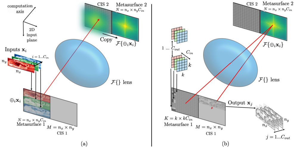
The image presents two diagrams, labeled (a) and (b), illustrating optical computing architectures using metasurfaces and lenses. Diagram (a) depicts the input stage, where multiple input images are combined and transformed by a lens and metasurface. Diagram (b) shows the output stage, where the transformed data is processed to generate output images.
### Components/Axes
**General Components:**
* **Computation Axis & 2D Input Plane:** An axis system indicating the direction of computation and the plane of input.
* **Inputs x<sub>i</sub>:** A stack of input images, indexed by *i* from 1 to C<sub>in</sub>, with dimensions n<sub>x</sub> and n<sub>y</sub>.
* **Metasurface 1:** A surface with dimensions N = n<sub>x</sub> * n<sub>y</sub> * C<sub>in</sub>.
* **CIS 1:** Computational Imaging System 1, with dimensions M = n<sub>x</sub> * n<sub>y</sub>.
* **Lens:** A lens element, denoted as F{}.
* **Metasurface 2:** A surface with dimensions N = n<sub>x</sub> * n<sub>y</sub> * C<sub>in</sub>.
* **CIS 2:** Computational Imaging System 2.
* **Outputs x<sub>j</sub>:** A stack of output images, indexed by *j* from 1 to C<sub>out</sub>, with dimensions n<sub>x</sub> and n<sub>y</sub>.
**Diagram (a) Specifics:**
* **⊕<sub>i</sub>x<sub>i</sub>:** Represents the combination of input images.
* **Copy:** Indicates that the Fourier transform of the combined input is copied to Metasurface 2.
* **F{⊕<sub>i</sub>x<sub>i</sub>}:** Represents the Fourier transform of the combined input images.
**Diagram (b) Specifics:**
* **1 ... C<sub>out</sub>:** Indicates the range of output channels.
* **C<sub>in</sub>:** Indicates the number of input channels.
* **k:** Represents a kernel or filter.
* **K = k x k C<sub>in</sub>:** Represents the dimensions of Metasurface 1.
* **Output x<sub>j</sub>:** Represents the output images.
### Detailed Analysis
**Diagram (a): Input Stage**
1. **Inputs x<sub>i</sub>:** A series of input images, represented by stacked rectangles colored red, green, and blue, indicating multiple input channels (i = 1...C<sub>in</sub>). The dimensions of each input image are n<sub>x</sub> and n<sub>y</sub>.
2. **⊕<sub>i</sub>x<sub>i</sub>:** The input images are combined (summed or concatenated) into a single representation.
3. **Metasurface 1:** The combined input is projected onto Metasurface 1, which has dimensions N = n<sub>x</sub> * n<sub>y</sub> * C<sub>in</sub>. A portion of Metasurface 1 is labeled CIS 1, with dimensions M = n<sub>x</sub> * n<sub>y</sub>.
4. **Lens:** The combined input is passed through a lens, denoted as F{}.
5. **Metasurface 2:** The Fourier transform of the combined input, F{⊕<sub>i</sub>x<sub>i</sub>}, is copied to Metasurface 2, which has dimensions N = n<sub>x</sub> * n<sub>y</sub> * C<sub>in</sub>. The left portion of Metasurface 2 is labeled CIS 2.
**Diagram (b): Output Stage**
1. **Input from Lens:** The Fourier transformed data from the lens, F{⊕<sub>i</sub>x<sub>i</sub>}, is projected onto Metasurface 2.
2. **Kernel Operation:** A series of kernels (k) are applied to the data, indexed from 1 to C<sub>out</sub>.
3. **Metasurface 1:** The result of the kernel operation is projected onto Metasurface 1, which has dimensions K = k x k C<sub>in</sub>. A portion of Metasurface 1 is labeled CIS 1, with dimensions M = n<sub>x</sub> * n<sub>y</sub>.
4. **Output x<sub>j</sub>:** The processed data is transformed into a series of output images, indexed by *j* from 1 to C<sub>out</sub>, with dimensions n<sub>x</sub> and n<sub>y</sub>.
### Key Observations
* Both diagrams utilize a lens to perform a Fourier transform on the input data.
* Metasurfaces are used to manipulate the data in both the input and output stages.
* The dimensions of the metasurfaces are related to the dimensions of the input images and the number of input channels.
* Diagram (a) focuses on the input and Fourier transform, while diagram (b) focuses on the kernel operation and output generation.
### Interpretation
The diagrams illustrate two stages of an optical computing architecture. Diagram (a) shows how multiple input images are combined and transformed into the frequency domain using a lens and metasurface. Diagram (b) shows how the transformed data is processed using kernels and another metasurface to generate multiple output images. The architecture leverages the properties of light and optical elements to perform complex computations in a potentially more efficient manner than traditional electronic computing. The use of metasurfaces allows for precise control over the manipulation of light, enabling the implementation of various computational operations. The diagrams highlight the flow of data through the system and the key components involved in the optical computing process.