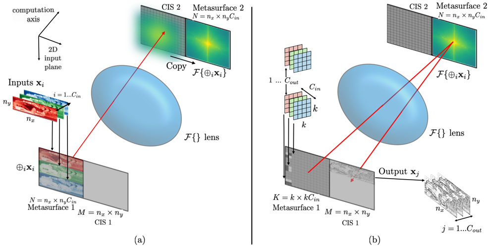
\n ## Technical Diagram: Optical Metasurface Computing Architectures ### Overview The image displays two technical diagrams, labeled (a) and (b), illustrating conceptual architectures for optical computing or signal processing systems. Both diagrams depict a process where input data is modulated by a first metasurface, transformed by a lens (representing a Fourier transform operation, ℱ{}), and then processed by a second metasurface or detected. The diagrams use a combination of 3D-rendered components, 2D planes, and mathematical notation to explain the data flow and physical transformations. ### Components/Axes **Common Elements in Both Diagrams:** * **Computation Axis:** A 3D coordinate system shown in the top-left of (a), defining the spatial orientation. * **2D Input Plane:** The plane from which input data originates. * **ℱ{} lens:** A large, blue, ellipsoidal element representing an optical lens that performs a Fourier transform (ℱ) on the light field passing through it. * **Metasurface 1:** A planar optical element that modulates the incoming light. It has dimensions labeled `N = n_x × n_y C_in` and `M = n_x × n_y`. * **CIS 1:** A planar element adjacent to Metasurface 1, likely a Coherent Image Sensor or similar detector plane. * **Metasurface 2:** A second planar optical element positioned after the lens. It has dimensions labeled `N = n_x × n_y C_in`. * **CIS 2:** A planar element adjacent to Metasurface 2. * **Mathematical Notation `ℱ{⊕_i x_i}`:** Appears near Metasurface 2 in both diagrams, indicating the Fourier transform of the concatenated input signals. **Diagram (a) Specifics:** * **Inputs `x_i`:** A stack of colored 2D input planes (red, green, blue) labeled `i = 1...C_in`. Each plane has spatial dimensions `n_x` and `n_y`. * **Concatenation Symbol `⊕_i x_i`:** Shows the vertical stacking of the `C_in` input channels into a single taller plane before Metasurface 1. * **"Copy" Arrow:** A red arrow points from the output plane after the lens to Metasurface 2, with the label "Copy". **Diagram (b) Specifics:** * **Kernel/Filter Stack:** A stack of small 2D grids (colored pink, green, blue) labeled `1 ... C_out` and `C_in`, with a spatial size `k`. This represents convolutional kernels or filters. * **Kernel Application:** Arrows show these kernels being applied to the input data path before Metasurface 1. * **Metasurface 1 Label:** In (b), Metasurface 1 is labeled with `K = k × k C_in`, indicating its role in implementing the kernel operation. * **Output `x_j`:** A 3D volume of data (a stack of 2D planes) labeled `j = 1...C_out`, with spatial dimensions `n_x` and `n_y`. An arrow labeled "Output `x_j`" points from CIS 1 to this volume. * **Red Ray Tracing:** Two red lines trace paths from the kernel stack, through the lens, to a focal point on Metasurface 2, illustrating the optical implementation of a mathematical operation (likely convolution via Fourier optics). ### Detailed Analysis **Diagram (a) Flow:** 1. **Input Stage:** `C_in` separate 2D input channels (`x_i`), each of size `n_x × n_y`, are vertically concatenated (`⊕_i`) to form a single tall input plane. 2. **First Modulation:** This concatenated plane illuminates **Metasurface 1**. 3. **Fourier Transform:** The modulated light passes through the **ℱ{} lens**, which optically computes the Fourier transform of the input field. 4. **Processing/Detection:** The transformed field interacts with **Metasurface 2** and/or is detected by **CIS 2**. The label "Copy" and the notation `ℱ{⊕_i x_i}` suggest the system may be performing a direct transfer or replication of the Fourier-domain representation. **Diagram (b) Flow:** 1. **Kernel-Input Interaction:** A set of `C_out` kernels, each of size `k × k × C_in`, is applied to the input data stream. This is depicted as the kernel stack interacting with the input path. 2. **First Modulation:** The result of this interaction (likely a correlation or convolution operation) is encoded onto **Metasurface 1** (now labeled `K = k × k C_in`). 3. **Fourier Transform & Filtering:** Light from Metasurface 1 passes through the **ℱ{} lens**. The red ray tracing indicates that the kernel information is optically combined with the input in the Fourier domain at the plane of **Metasurface 2**. 4. **Output Generation:** The processed signal is detected at **CIS 1** and read out as a 4D output tensor `x_j` with dimensions `C_out × n_x × n_y`. ### Key Observations 1. **Architectural Progression:** Diagram (a) appears to show a basic optical Fourier transform setup, while diagram (b) extends this to perform a more complex operation, likely a convolutional neural network (CNN) layer, using optical Fourier processing. 2. **Spatial Multiplexing:** Both systems use the vertical dimension (`C_in`) to handle multiple input channels in parallel within a single optical path. 3. **Fourier Domain Processing:** The central role of the lens (`ℱ{}`) highlights that the core computation happens in the spatial frequency (Fourier) domain, a key advantage of optical computing for operations like convolution. 4. **Component Mapping:** In (b), the physical **Metasurface 1** is explicitly mapped to the mathematical kernel operation (`K`), showing how a physical device implements a computational function. 5. **Output Dimensionality:** The final output in (b) is a multi-channel volume (`C_out`), consistent with the output of a convolutional layer in a neural network. ### Interpretation These diagrams illustrate the principle of **optical neural networks** or **diffractive deep neural networks (D²NN)**. They propose using specially engineered metasurfaces and the natural Fourier transforming property of lenses to perform massively parallel, low-energy computations. * **What it demonstrates:** The system in (b) is designed to execute a convolutional layer optically. The input channels and kernels are encoded into the wavefront of light. The lens performs the convolution's core operation—a multiplication in the Fourier domain—at the speed of light. Metasurface 2 likely acts as a learnable filter in this Fourier plane. The output is then captured by a sensor (CIS 1). * **Relationships:** The metasurfaces are the programmable "weights" of the optical network. The lens is the fixed "compute engine" that performs the transform. The spatial arrangement (`n_x, n_y, C_in, C_out`) directly mirrors the tensor dimensions used in digital deep learning. * **Notable Implications:** This approach promises extreme parallelism and energy efficiency for specific tasks like image processing, as the computation is performed by light propagation itself rather than by digital transistors. The diagrams serve as a conceptual blueprint for translating digital neural network operations into a physical, optical architecture. The shift from (a) to (b) shows the progression from a simple transform to a useful computational primitive (convolution).