# Technical Document Extraction: 3D Spatial Estimation Plot
## 1. Component Isolation
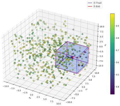
The image is a 3D scatter plot visualizing a dataset within a coordinate system, featuring two overlapping bounding boxes and a color-coded intensity scale.
* **Header/Legend Region:** Top right corner.
* **Main Chart Region:** Central 3D coordinate space.
* **Colorbar Region:** Far right vertical axis.
---
## 2. Metadata and Legend Extraction
**Spatial Grounding [x, y]:** The legend is located in the upper right quadrant of the image frame.
| Label | Visual Representation | Description |
| :--- | :--- | :--- |
| **$S$ (True)** | Solid Blue Line | Represents the ground truth spatial volume (True set). |
| **$\hat{S}$ (Est)** | Solid Red Line | Represents the estimated spatial volume (Estimated set). |
---
## 3. Axis and Coordinate System
The plot uses a Cartesian 3D coordinate system with the following scales:
* **$x_0$ Axis (Bottom Left):** Ranges from **-10.0 to 10.0** with increments of 2.5.
* **$x_1$ Axis (Bottom Right):** Ranges from **-10.0 to 10.0** with increments of 2.5.
* **$x_2$ Axis (Vertical):** Ranges from **-10.0 to 10.0** with increments of 2.5.
---
## 4. Data Series and Trends
### A. Scatter Plot (Data Points)
* **Distribution:** Points are distributed throughout the 3D volume, primarily concentrated between -10 and 10 on all axes.
* **Color Encoding:** Points are colored based on a value scale (likely probability or density).
* **Trend:** Points outside the bounding boxes generally appear in the yellow-to-green range (higher values on the colorbar). Points inside the blue/red bounding boxes transition into darker purple/blue shades (lower values on the colorbar).
* **Colorbar Scale:**
* **Range:** 0.4 to 0.9.
* **Gradient:** Dark Purple (0.4) $\rightarrow$ Teal (0.6) $\rightarrow$ Green (0.8) $\rightarrow$ Yellow (0.9).
### B. Bounding Volumes (The Cuboids)
* **$S$ (True) - Blue Box:**
* **Trend:** A semi-transparent blue cuboid located in the positive $x_0$, positive $x_1$, and negative $x_2$ octant.
* **Approximate Bounds:**
* $x_0$: ~[2.5, 10.0]
* $x_1$: ~[0.0, 7.5]
* $x_2$: ~[-7.5, 2.5]
* **$\hat{S}$ (Est) - Red Box:**
* **Trend:** A red wireframe/outline cuboid that closely overlaps the blue box.
* **Observation:** The red box appears slightly larger or shifted along the $x_1$ and $x_2$ axes compared to the blue box, indicating a high-accuracy estimation with minor marginal error.
---
## 5. Technical Summary
This visualization depicts a 3D point cloud where a specific subset of data (characterized by lower values, ~0.4 - 0.5) is being isolated. The **True Volume ($S$)** defines the actual region containing these low-value points. The **Estimated Volume ($\hat{S}$)** shows the result of a model's attempt to bound that same region. The high degree of overlap between the blue solid volume and the red outline suggests the estimation algorithm is performing with high precision.