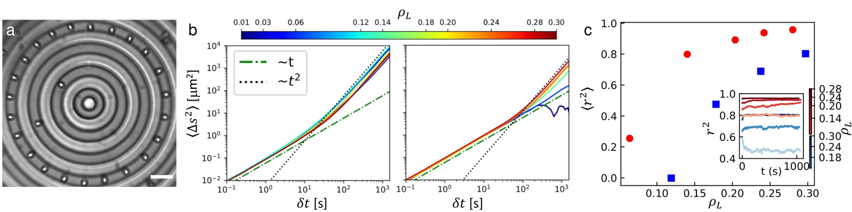
## Composite Figure: Particle Dynamics in Confined Environments ### Overview The image presents a composite figure analyzing particle dynamics within a confined environment. It consists of three sub-figures: (a) a microscopic image of the confinement structure, (b) two plots showing the mean squared displacement (MSD) of particles as a function of time, color-coded by particle density, and (c) a plot showing the time-averaged MSD as a function of particle density, with an inset showing the time evolution of the MSD for different densities. ### Components/Axes **Sub-figure a:** * **Description:** A grayscale microscopic image showing a circular confinement structure with concentric rings. Particles (appearing as small bright dots) are trapped within the rings. * **Scale Bar:** A white scale bar is visible in the bottom right corner. **Sub-figure b (Left and Right Plots):** * **Y-axis:** `<Δs²> [µm²]` - Mean squared displacement, plotted on a logarithmic scale from approximately 10^-2 to 10^4. * **X-axis:** `δt [s]` - Time interval, plotted on a logarithmic scale from approximately 10^-1 to 10^3. * **Color Bar (Top):** `ρL` - Particle density, ranging from 0.01 (blue) to 0.30 (red). The color gradient is as follows: 0.01 (dark blue), 0.03 (blue), 0.06 (light blue), 0.12 (cyan), 0.14 (light green), 0.18 (yellow-green), 0.20 (yellow), 0.24 (orange), 0.28 (red-orange), 0.30 (red). * **Reference Lines:** * Green dashed-dotted line: Labeled "~t". * Black dotted line: Labeled "~t²". * **Data Series:** Each colored line represents the MSD for a specific particle density (ρL), as indicated by the color bar. **Sub-figure c:** * **Y-axis:** `<r²>` - Time-averaged mean squared displacement, plotted on a linear scale from 0.0 to 1.0. * **X-axis:** `ρL` - Particle density, plotted on a linear scale from 0.10 to 0.30. * **Data Points:** * Red circles: Represent one data series. * Blue squares: Represent another data series. * **Inset Plot:** * Y-axis: `r^2` - Mean squared displacement, plotted on a linear scale from approximately 0.4 to 1.0. * X-axis: `t (s)` - Time, plotted on a linear scale from 0 to 1000. * Data Series: Colored lines representing the time evolution of the MSD for different particle densities (ρL), matching the color scheme in sub-figure b. ### Detailed Analysis **Sub-figure b (MSD vs. Time):** * **General Trend:** For all densities, the MSD increases with time. At short times, the MSD follows a t² relationship, indicating ballistic motion. At longer times, the MSD transitions to a t relationship, indicating diffusive motion. * **Density Dependence:** * **ρL = 0.01 (Dark Blue):** The MSD initially follows the t² line, then transitions to a slope slightly below the t line at longer times. * **ρL = 0.03 (Blue):** Similar to ρL = 0.01, but with a slightly higher MSD. * **ρL = 0.06 (Light Blue):** The MSD is higher than the previous two densities and follows a similar trend. * **ρL = 0.12 (Cyan):** The MSD continues to increase. * **ρL = 0.14 (Light Green):** The MSD continues to increase. * **ρL = 0.18 (Yellow-Green):** The MSD continues to increase. * **ρL = 0.20 (Yellow):** The MSD continues to increase. * **ρL = 0.24 (Orange):** The MSD continues to increase. * **ρL = 0.28 (Red-Orange):** The MSD continues to increase. * **ρL = 0.30 (Red):** The MSD is the highest among all densities and follows a similar trend. * **Crossover:** The point at which the MSD transitions from t² to t behavior shifts to shorter times as the density increases. **Sub-figure c (Time-Averaged MSD vs. Density):** * **Red Circles:** The time-averaged MSD (represented by red circles) increases with density from ρL = 0.10 to ρL = 0.24, then decreases slightly at ρL = 0.30. Approximate values: * ρL = 0.10, <r²> ≈ 0.25 * ρL = 0.18, <r²> ≈ 0.75 * ρL = 0.24, <r²> ≈ 0.95 * ρL = 0.30, <r²> ≈ 0.90 * **Blue Squares:** The time-averaged MSD (represented by blue squares) is low at ρL = 0.10 and increases to a maximum at ρL = 0.30. Approximate values: * ρL = 0.10, <r²> ≈ 0.0 * ρL = 0.18, <r²> ≈ 0.45 * ρL = 0.24, <r²> ≈ 0.70 * ρL = 0.30, <r²> ≈ 0.80 * **Inset Plot:** The inset plot shows that the MSD reaches a plateau at longer times for all densities. The plateau value increases with density, consistent with the trend observed in the main plot. ### Key Observations * The MSD of particles in the confined environment depends on both time and particle density. * At short times, the motion is ballistic, while at longer times, it is diffusive. * The time-averaged MSD exhibits a non-monotonic dependence on density, with a peak at intermediate densities for the red circle data series. * The inset plot confirms that the MSD reaches a steady-state value at long times. ### Interpretation The data suggests that particle dynamics in the confined environment are influenced by crowding effects. At low densities, particles can move freely, resulting in a higher MSD. As the density increases, crowding becomes more significant, hindering particle movement and reducing the MSD. However, at very high densities, the particles may become trapped in local minima, leading to a slight increase in the MSD. The two data series in sub-figure c likely represent different types of particles or different methods of calculating the MSD, leading to the observed differences in their density dependence. The confinement structure and particle interactions play a crucial role in determining the overall dynamics.