## Line Chart: Median TTS vs Problem Size
### Overview
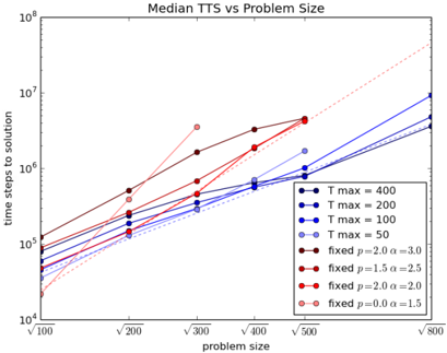
This is a log-log line chart comparing the median "Time To Solution" (TTS) in time steps against increasing problem sizes for different algorithmic parameter settings. The chart demonstrates how computational effort scales with problem complexity under various configurations.
### Components/Axes
* **Chart Title:** "Median TTS vs Problem Size" (Top Center)
* **Y-Axis:**
* **Label:** "time steps to solution" (Left side, rotated vertically)
* **Scale:** Logarithmic (base 10), ranging from 10² to 10⁸.
* **Major Ticks:** 10², 10³, 10⁴, 10⁵, 10⁶, 10⁷, 10⁸.
* **X-Axis:**
* **Label:** "problem size" (Bottom Center)
* **Scale:** Appears to be a linear scale of the square root of the problem size, with markers at specific points.
* **Major Tick Labels:** √100, √200, √300, √400, √500, √800.
* **Legend:** Positioned in the bottom-right quadrant of the chart area. It contains two distinct groups of data series.
* **Group 1 (Blue Lines - "T max" series):**
* Solid blue line with filled circle markers: `T max = 400`
* Dashed blue line with filled circle markers: `T max = 200`
* Solid blue line with open circle markers: `T max = 100`
* Dashed blue line with open circle markers: `T max = 50`
* **Group 2 (Red/Brown Lines - "fixed p, α" series):**
* Solid dark brown line with filled circle markers: `fixed p=2.0 α=3.0`
* Dashed dark red line with filled circle markers: `fixed p=1.5 α=2.5`
* Solid red line with open circle markers: `fixed p=2.0 α=2.0`
* Dashed light red/pink line with open circle markers: `fixed p=0.0 α=1.5`
### Detailed Analysis
**Data Series Trends and Approximate Points:**
All series show a positive correlation: as problem size increases, the median time steps to solution increase. The relationship appears roughly linear on this log-log plot, suggesting a power-law relationship (TTS ∝ (problem size)^k).
**Group 1: T max Series (Blue)**
* **T max = 400 (Solid Blue, Filled Circles):** The highest line in this group. Starts near 10³ steps at √100, rises to approximately 10⁵ steps at √500, and ends near 10⁷ steps at √800.
* **T max = 200 (Dashed Blue, Filled Circles):** Runs parallel but below the T max=400 line. Starts ~8x10² at √100, reaches ~5x10⁴ at √500, and ~5x10⁶ at √800.
* **T max = 100 (Solid Blue, Open Circles):** Below the previous two. Starts ~5x10² at √100, ~2x10⁴ at √500, and ~2x10⁶ at √800.
* **T max = 50 (Dashed Blue, Open Circles):** The lowest blue line. Starts ~2x10² at √100, ~8x10³ at √500, and ~8x10⁵ at √800.
* **Trend:** Within this group, a higher `T max` value consistently results in a higher median TTS for the same problem size. The lines are roughly parallel, indicating similar scaling exponents.
**Group 2: Fixed p, α Series (Red/Brown)**
* **fixed p=2.0 α=3.0 (Solid Brown, Filled Circles):** The steepest and ultimately highest line on the chart. Starts near 10³ at √100, crosses above the T max=400 line between √200 and √300, and reaches nearly 10⁷ by √500 (data does not extend to √800).
* **fixed p=1.5 α=2.5 (Dashed Dark Red, Filled Circles):** Starts near 10³ at √100, similar to the brown line. It rises less steeply, reaching ~4x10⁵ at √500.
* **fixed p=2.0 α=2.0 (Solid Red, Open Circles):** Starts lower, around 5x10² at √100. Rises to ~2x10⁵ at √500.
* **fixed p=0.0 α=1.5 (Dashed Pink, Open Circles):** The lowest line on the entire chart for most of the range. Starts near 10² at √100, rises to ~10⁴ at √300, and ~10⁵ at √500.
* **Trend:** A higher `α` value correlates with a steeper slope (worse scaling). The line for `α=3.0` has the most aggressive growth. The ordering of lines by `α` value (3.0 > 2.5 > 2.0 > 1.5) is consistent with their vertical ordering at larger problem sizes.
### Key Observations
1. **Two Distinct Scaling Families:** The chart clearly separates into two groups of strategies: those varying a `T max` parameter (blue) and those with fixed `p` and `α` parameters (red/brown).
2. **Crossover Point:** The `fixed p=2.0 α=3.0` strategy, while starting at a similar level to the `T max` strategies for small problems (√100), scales much more poorly and becomes the most computationally expensive option for problems larger than approximately √250.
3. **Consistent Ordering:** Within each group, the performance ordering of the parameter settings is consistent across all problem sizes shown.
4. **Power-Law Behavior:** The near-linear trends on the log-log plot strongly suggest that the median TTS follows a power-law relationship with the problem size for all tested configurations.
### Interpretation
This chart is a performance benchmark comparing different algorithmic approaches or parameterizations for a computational problem. The "problem size" likely refers to the scale of the input (e.g., number of variables, graph nodes).
* **The "T max" strategies (blue)** appear to represent a family of algorithms where a maximum time or iteration limit (`T max`) is a key parameter. Higher limits allow for more computation, leading to higher median TTS but potentially better solution quality (not shown). Their parallel scaling suggests they share the same fundamental complexity class.
* **The "fixed p, α" strategies (red/brown)** likely represent a different algorithmic family where `p` and `α` are tuning parameters (e.g., for a probabilistic or heuristic method). The parameter `α` has a dramatic effect on scalability. The `α=3.0` setting leads to prohibitively expensive scaling for large problems, while `α=1.5` offers the best scalability in this group but may come with trade-offs in other metrics like solution accuracy.
* **Practical Implication:** For small problems (√100-√200), the choice of strategy has a smaller impact on runtime. However, for large-scale problems (√500 and beyond), selecting a strategy with good scaling (low `α` or a moderate `T max`) is critical to avoid exponential growth in computation time. The `fixed p=0.0 α=1.5` configuration shows the most favorable scaling among the fixed-parameter group, while among the `T max` group, lower `T max` values scale better but may be insufficient for finding solutions. The optimal choice depends on the required problem size and acceptable time budget.