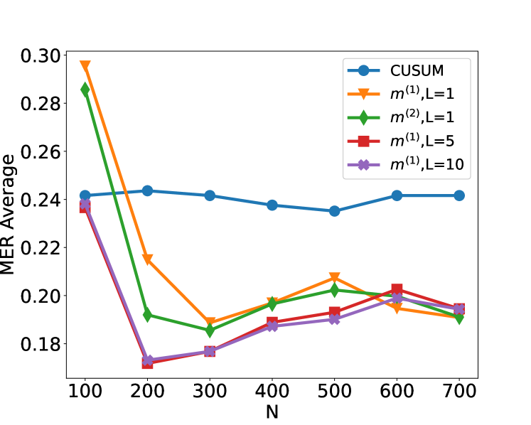
## Line Chart: MER Average vs N ### Overview The image is a line chart comparing the MER (Minimum Error Rate) Average for different algorithms (CUSUM, m^(1), m^(2)) with varying parameters (L=1, L=5, L=10) against the variable N. The chart displays how the MER Average changes as N increases from 100 to 700. ### Components/Axes * **X-axis:** N, ranging from 100 to 700 in increments of 100. * **Y-axis:** MER Average, ranging from 0.18 to 0.30 in increments of 0.02. * **Legend (Top-Right):** * Blue line with circle markers: CUSUM * Orange line with triangle markers: m^(1), L=1 * Green line with diamond markers: m^(2), L=1 * Red line with square markers: m^(1), L=5 * Purple line with pentagon markers: m^(1), L=10 ### Detailed Analysis * **CUSUM (Blue):** The MER Average starts at approximately 0.24 at N=100, remains relatively stable between 0.24 and 0.235 from N=200 to N=500, then increases slightly to approximately 0.24 at N=600 and remains at 0.24 at N=700. * N=100: 0.24 * N=200: 0.243 * N=300: 0.242 * N=400: 0.241 * N=500: 0.236 * N=600: 0.242 * N=700: 0.242 * **m^(1), L=1 (Orange):** The MER Average starts at approximately 0.29 at N=100, decreases sharply to approximately 0.215 at N=200, then decreases further to approximately 0.19 at N=300. It then increases to approximately 0.198 at N=400, then increases further to approximately 0.208 at N=500, then decreases to approximately 0.20 at N=600, and finally decreases to approximately 0.195 at N=700. * N=100: 0.29 * N=200: 0.215 * N=300: 0.19 * N=400: 0.198 * N=500: 0.208 * N=600: 0.20 * N=700: 0.195 * **m^(2), L=1 (Green):** The MER Average starts at approximately 0.285 at N=100, decreases sharply to approximately 0.19 at N=200, then decreases slightly to approximately 0.185 at N=300. It then increases to approximately 0.198 at N=400, then increases slightly to approximately 0.198 at N=500, then increases slightly to approximately 0.20 at N=600, and finally decreases to approximately 0.19 at N=700. * N=100: 0.285 * N=200: 0.19 * N=300: 0.185 * N=400: 0.198 * N=500: 0.198 * N=600: 0.20 * N=700: 0.19 * **m^(1), L=5 (Red):** The MER Average starts at approximately 0.235 at N=100, decreases sharply to approximately 0.17 at N=200, then increases slightly to approximately 0.177 at N=300. It then increases to approximately 0.188 at N=400, then increases slightly to approximately 0.19 at N=500, then increases to approximately 0.202 at N=600, and finally decreases to approximately 0.195 at N=700. * N=100: 0.235 * N=200: 0.17 * N=300: 0.177 * N=400: 0.188 * N=500: 0.19 * N=600: 0.202 * N=700: 0.195 * **m^(1), L=10 (Purple):** The MER Average starts at approximately 0.238 at N=100, decreases sharply to approximately 0.172 at N=200, then increases slightly to approximately 0.177 at N=300. It then increases to approximately 0.188 at N=400, then increases slightly to approximately 0.19 at N=500, then increases to approximately 0.20 at N=600, and finally decreases to approximately 0.192 at N=700. * N=100: 0.238 * N=200: 0.172 * N=300: 0.177 * N=400: 0.188 * N=500: 0.19 * N=600: 0.20 * N=700: 0.192 ### Key Observations * The CUSUM algorithm (blue line) has a relatively stable MER Average across the range of N values, with a slight increase at N=600. * The m^(1), L=1 (orange line) and m^(2), L=1 (green line) algorithms show a sharp decrease in MER Average from N=100 to N=200, followed by a gradual increase and then a slight decrease. * The m^(1), L=5 (red line) and m^(1), L=10 (purple line) algorithms show a sharp decrease in MER Average from N=100 to N=200, followed by a gradual increase and then a slight decrease. * For N values greater than 200, the m^(1), L=5 and m^(1), L=10 algorithms have the lowest MER Average. ### Interpretation The chart suggests that the CUSUM algorithm is more stable across different values of N, while the other algorithms (m^(1), m^(2)) are more sensitive to changes in N, particularly at lower values. The algorithms m^(1), L=5 and m^(1), L=10 appear to perform better (lower MER Average) for N values greater than 200. The initial sharp decrease in MER Average for m^(1) and m^(2) algorithms indicates that increasing N from 100 to 200 significantly improves their performance. The subsequent gradual increase and slight decrease suggest that there is an optimal range of N values for these algorithms.

## Line Chart: MER Average vs. N for Different Methods ### Overview This image displays a line chart comparing the "MER Average" on the y-axis against "N" on the x-axis for five different methods: CUSUM, $m^{(1), L=1}$, $m^{(2), L=1}$, $m^{(1), L=5}$, and $m^{(1), L=10}$. The chart shows how the MER Average changes as N increases for each of these methods. ### Components/Axes * **Chart Type**: Line Chart * **Title**: Not explicitly stated, but implied by the axes and legend. * **X-axis**: * **Label**: N * **Scale**: Numerical, ranging from 100 to 700. * **Markers**: 100, 200, 300, 400, 500, 600, 700. * **Y-axis**: * **Label**: MER Average * **Scale**: Numerical, ranging from approximately 0.18 to 0.30. * **Markers**: 0.18, 0.20, 0.22, 0.24, 0.26, 0.28, 0.30. * **Legend**: Located in the top-right quadrant of the chart. * **CUSUM**: Blue line with circular markers. * **$m^{(1), L=1}$**: Orange line with triangular markers. * **$m^{(2), L=1}$**: Green line with diamond markers. * **$m^{(1), L=5}$**: Red line with square markers. * **$m^{(1), L=10}$**: Purple line with cross markers. ### Detailed Analysis **Data Series Trends and Points:** 1. **CUSUM (Blue, Circles)**: * **Trend**: The CUSUM line starts at approximately 0.242 at N=100, then slightly increases to around 0.244 at N=200, remains relatively stable between 0.240 and 0.242 from N=300 to N=500, then increases slightly to approximately 0.243 at N=600, and finally stays at approximately 0.242 at N=700. Overall, it shows a relatively flat trend with minor fluctuations. * **Approximate Data Points**: * N=100: 0.242 * N=200: 0.244 * N=300: 0.240 * N=400: 0.238 * N=500: 0.237 * N=600: 0.243 * N=700: 0.242 2. **$m^{(1), L=1}$ (Orange, Triangles)**: * **Trend**: This line starts at a high value of approximately 0.298 at N=100. It then drops sharply to approximately 0.215 at N=200. The trend continues downwards to approximately 0.195 at N=300. After N=300, it begins to increase, reaching approximately 0.200 at N=400, then 0.210 at N=500, and 0.202 at N=600. Finally, it decreases slightly to approximately 0.195 at N=700. * **Approximate Data Points**: * N=100: 0.298 * N=200: 0.215 * N=300: 0.195 * N=400: 0.200 * N=500: 0.210 * N=600: 0.202 * N=700: 0.195 3. **$m^{(2), L=1}$ (Green, Diamonds)**: * **Trend**: This line starts at approximately 0.285 at N=100. It then decreases sharply to approximately 0.192 at N=200. The trend continues downwards to approximately 0.185 at N=300. After N=300, it begins to increase, reaching approximately 0.198 at N=400, then 0.205 at N=500, and 0.195 at N=600. Finally, it decreases slightly to approximately 0.192 at N=700. * **Approximate Data Points**: * N=100: 0.285 * N=200: 0.192 * N=300: 0.185 * N=400: 0.198 * N=500: 0.205 * N=600: 0.195 * N=700: 0.192 4. **$m^{(1), L=5}$ (Red, Squares)**: * **Trend**: This line starts at approximately 0.240 at N=100. It then drops sharply to approximately 0.175 at N=200. The trend continues slightly upwards to approximately 0.177 at N=300, then to 0.185 at N=400, and 0.198 at N=500. It then increases to approximately 0.202 at N=600, before decreasing to approximately 0.195 at N=700. * **Approximate Data Points**: * N=100: 0.240 * N=200: 0.175 * N=300: 0.177 * N=400: 0.185 * N=500: 0.198 * N=600: 0.202 * N=700: 0.195 5. **$m^{(1), L=10}$ (Purple, Crosses)**: * **Trend**: This line starts at approximately 0.238 at N=100. It then drops sharply to approximately 0.175 at N=200. The trend continues slightly upwards to approximately 0.178 at N=300, then to 0.190 at N=400, and 0.195 at N=500. It then decreases slightly to approximately 0.192 at N=600, before decreasing further to approximately 0.190 at N=700. * **Approximate Data Points**: * N=100: 0.238 * N=200: 0.175 * N=300: 0.178 * N=400: 0.190 * N=500: 0.195 * N=600: 0.192 * N=700: 0.190 ### Key Observations * **Initial High Values**: The methods $m^{(1), L=1}$ and $m^{(2), L=1}$ exhibit significantly higher MER Average values at N=100 compared to CUSUM, $m^{(1), L=5}$, and $m^{(1), L=10}$. * **Sharp Decrease**: All methods except CUSUM show a dramatic decrease in MER Average from N=100 to N=200. * **Convergence**: For N values greater than or equal to 300, the MER Average values for $m^{(1), L=1}$, $m^{(2), L=1}$, $m^{(1), L=5}$, and $m^{(1), L=10}$ tend to converge, fluctuating within a narrower range (approximately 0.175 to 0.210). * **CUSUM Stability**: The CUSUM method maintains a relatively stable MER Average throughout the observed range of N, hovering around 0.24. * **Lowest MER Average**: The methods $m^{(1), L=5}$ and $m^{(1), L=10}$ achieve the lowest MER Average values, particularly around N=200 and N=300, with values as low as approximately 0.175. * **Crossings**: The lines for $m^{(1), L=5}$ and $m^{(1), L=10}$ are very close for most of the N range, with slight crossings occurring. Similarly, $m^{(1), L=1}$ and $m^{(2), L=1}$ also show some proximity in their trends after the initial drop. ### Interpretation The chart demonstrates the performance of different methods (CUSUM and various $m$ functions with different parameters L) in terms of their "MER Average" as the sample size "N" increases. * **Initial Performance**: At a small sample size (N=100), $m^{(1), L=1}$ and $m^{(2), L=1}$ appear to be less optimal, showing very high MER Averages. This could indicate that these methods are more sensitive to initial data or require more data to stabilize. CUSUM, $m^{(1), L=5}$, and $m^{(1), L=10}$ perform better at N=100. * **Adaptability**: The sharp decline in MER Average for most methods from N=100 to N=200 suggests that they become more efficient or accurate as more data becomes available. This is a common characteristic of many statistical or machine learning methods. * **Long-term Behavior**: For larger N, the convergence of $m^{(1), L=1}$, $m^{(2), L=1}$, $m^{(1), L=5}$, and $m^{(1), L=10}$ indicates that their performance becomes similar. The choice between these methods might then depend on other factors not shown in this chart, such as computational cost or specific error profiles. * **CUSUM's Consistency**: The CUSUM method's stable performance across different N values suggests it is robust and less affected by sample size variations. However, its MER Average is consistently higher than the other methods for N > 200. This implies that while CUSUM is stable, it might not be as efficient in minimizing the MER Average as the other methods when sufficient data is available. * **Parameter Impact**: Comparing $m^{(1), L=5}$ and $m^{(1), L=10}$, their performance is very similar, suggesting that increasing L from 5 to 10 for the $m^{(1)}$ method has a minimal impact on the MER Average in this context. The slight differences might be within the margin of error or represent minor trade-offs. In essence, the chart suggests that for achieving a low MER Average, methods like $m^{(1), L=5}$ and $m^{(1), L=10}$ are effective, especially with increasing N. CUSUM offers stability but at a higher MER Average. The initial high values for $m^{(1), L=1}$ and $m^{(2), L=1}$ at small N highlight the importance of sample size for these specific configurations.

## Line Chart: MER Average vs. N for Different Algorithms ### Overview This image presents a line chart comparing the Mean Error Rate (MER) Average for different algorithms as a function of 'N'. The algorithms are CUSUM, m⁽¹⁾ with L=1, m⁽²⁾ with L=1, m⁽¹⁾ with L=5, and m⁽¹⁾ with L=10. The chart displays how the MER Average changes as 'N' increases from 100 to 700. ### Components/Axes * **X-axis:** Labeled "N". Scale ranges from approximately 100 to 700, with markers at 100, 200, 300, 400, 500, 600, and 700. * **Y-axis:** Labeled "MER Average". Scale ranges from approximately 0.18 to 0.30, with markers at 0.18, 0.20, 0.22, 0.24, 0.26, 0.28, and 0.30. * **Legend:** Located in the top-right corner. Contains the following labels and corresponding colors: * CUSUM (Blue) * m⁽¹⁾, L=1 (Orange) * m⁽²⁾, L=1 (Green) * m⁽¹⁾, L=5 (Red) * m⁽¹⁾, L=10 (Purple) ### Detailed Analysis * **CUSUM (Blue Line):** The line starts at approximately 0.245 at N=100, decreases slightly to around 0.24 at N=200, remains relatively stable around 0.24 to 0.25 until N=600, and then increases slightly to approximately 0.245 at N=700. * **m⁽¹⁾, L=1 (Orange Line):** This line exhibits a steep downward trend from N=100 to N=200, decreasing from approximately 0.29 to 0.19. It then fluctuates between approximately 0.19 and 0.21 from N=200 to N=700. * **m⁽²⁾, L=1 (Green Line):** The line starts at approximately 0.25 at N=100, decreases to around 0.21 at N=200, increases to approximately 0.215 at N=400, and then decreases slightly to around 0.205 at N=700. * **m⁽¹⁾, L=5 (Red Line):** This line shows a very steep decrease from approximately 0.29 at N=100 to approximately 0.16 at N=200. It then remains relatively stable, fluctuating between approximately 0.16 and 0.18 from N=200 to N=700. * **m⁽¹⁾, L=10 (Purple Line):** The line starts at approximately 0.25 at N=100, decreases to approximately 0.18 at N=200, and remains relatively stable, fluctuating between approximately 0.18 and 0.20 from N=200 to N=700. ### Key Observations * The algorithms m⁽¹⁾, L=5 and m⁽¹⁾, L=1 show the most significant initial decrease in MER Average as N increases from 100 to 200. * CUSUM exhibits the most stable MER Average across the range of N values. * m⁽¹⁾, L=1 and m⁽²⁾, L=1 show similar trends, but m⁽¹⁾, L=1 generally has a lower MER Average. * All algorithms converge to similar MER Average values as N approaches 700, with values between approximately 0.18 and 0.25. ### Interpretation The chart demonstrates the performance of different algorithms in terms of Mean Error Rate (MER) as the input size 'N' increases. The rapid initial decrease in MER Average for algorithms m⁽¹⁾, L=5 and m⁽¹⁾, L=1 suggests that these algorithms benefit significantly from larger input sizes, potentially due to improved statistical power or more accurate parameter estimation. The stability of the CUSUM algorithm indicates its robustness to changes in input size. The convergence of all algorithms at higher N values suggests that the algorithms achieve similar performance levels when sufficient data is available. The parameter 'L' appears to influence the performance of the m⁽¹⁾ algorithm, with smaller values of L (L=1) generally resulting in lower MER Averages compared to larger values (L=10). This could indicate that a smaller 'L' value allows for faster detection of changes or anomalies. The chart provides valuable insights into the trade-offs between different algorithms and the importance of input size in achieving optimal performance.

\n ## Line Chart: MER Average vs. N for Different Algorithms ### Overview The image is a line chart comparing the performance of five different algorithms or methods. The performance metric is "MER Average" plotted against a parameter "N". The chart shows how the average MER (likely Mean Error Rate or a similar metric) changes as N increases from 100 to 700 for each method. ### Components/Axes * **X-Axis:** Labeled "N". It has major tick marks at intervals of 100, ranging from 100 to 700. * **Y-Axis:** Labeled "MER Average". It has major tick marks at intervals of 0.02, ranging from 0.18 to 0.30. * **Legend:** Located in the top-right corner of the plot area. It contains five entries, each with a unique color, marker, and label: 1. Blue line with circle markers: `CUSUM` 2. Orange line with downward-pointing triangle markers: `m^{(1)}, L=1` 3. Green line with diamond markers: `m^{(2)}, L=1` 4. Red line with square markers: `m^{(1)}, L=5` 5. Purple line with 'x' markers: `m^{(1)}, L=10` ### Detailed Analysis **Trend Verification & Data Point Extraction (Approximate Values):** 1. **CUSUM (Blue, Circle):** * **Trend:** The line is relatively flat, showing only minor fluctuations. It starts around 0.24, dips slightly around N=500, and ends near its starting value. * **Data Points:** * N=100: ~0.242 * N=200: ~0.244 * N=300: ~0.242 * N=400: ~0.238 * N=500: ~0.235 * N=600: ~0.242 * N=700: ~0.242 2. **m^{(1)}, L=1 (Orange, Downward Triangle):** * **Trend:** Starts very high, drops sharply until N=300, then exhibits a fluctuating pattern with a local peak at N=500 before declining again. * **Data Points:** * N=100: ~0.296 (Highest point on the chart) * N=200: ~0.216 * N=300: ~0.190 * N=400: ~0.198 * N=500: ~0.208 * N=600: ~0.195 * N=700: ~0.192 3. **m^{(2)}, L=1 (Green, Diamond):** * **Trend:** Starts high, drops sharply until N=300, then shows a gradual, slightly fluctuating increase. * **Data Points:** * N=100: ~0.286 * N=200: ~0.192 * N=300: ~0.185 * N=400: ~0.196 * N=500: ~0.202 * N=600: ~0.198 * N=700: ~0.190 4. **m^{(1)}, L=5 (Red, Square):** * **Trend:** Starts moderately high, drops sharply to a minimum at N=200, then shows a steady, gradual increase. * **Data Points:** * N=100: ~0.236 * N=200: ~0.171 (Lowest point on the chart) * N=300: ~0.177 * N=400: ~0.189 * N=500: ~0.192 * N=600: ~0.203 * N=700: ~0.195 5. **m^{(1)}, L=10 (Purple, 'x'):** * **Trend:** Follows a very similar path to the red line (m^{(1)}, L=5), starting at a similar point, dropping to a minimum at N=200, and then gradually increasing, though it remains slightly below the red line for most points after N=300. * **Data Points:** * N=100: ~0.238 * N=200: ~0.173 * N=300: ~0.177 * N=400: ~0.187 * N=500: ~0.190 * N=600: ~0.200 * N=700: ~0.194 ### Key Observations 1. **Initial Performance Gap:** At the smallest N (100), there is a wide spread in performance. The `m^{(1)}, L=1` method has the highest MER (~0.296), while `CUSUM` and the `L=5`/`L=10` variants are clustered around ~0.24. 2. **Convergence at Low N:** All methods except `CUSUM` show a dramatic improvement (decrease in MER) as N increases from 100 to 200 or 300. The lowest overall MER values are achieved around N=200-300. 3. **CUSUM Stability:** The `CUSUM` method is an outlier in its behavior. It shows very little sensitivity to the parameter N, maintaining a nearly constant MER average between ~0.235 and ~0.244 across the entire range. 4. **Post-Convergence Behavior:** After N=300, the methods diverge again. The `m^{(1)}` variants (L=1,5,10) and `m^{(2)}, L=1` show a general trend of slightly increasing MER with N, while `CUSUM` remains flat. 5. **Effect of Parameter L:** For the `m^{(1)}` family, increasing L from 1 to 5 or 10 significantly improves performance (lowers MER) at small N (100-200). At larger N (≥400), the differences between L=5 and L=10 are minimal, and both are generally outperformed by `m^{(2)}, L=1`. ### Interpretation This chart likely compares the performance of different change-point detection or sequential analysis algorithms. "MER Average" is probably a measure of error or detection delay, where lower is better. "N" could represent sample size, sequence length, or a similar parameter. The data suggests a clear trade-off: * **CUSUM** is robust and stable, providing predictable, moderate performance regardless of N. It doesn't excel at any point but also doesn't degrade. * The **`m` methods** (likely referring to some multi-customer or multi-stream variant) are highly sensitive to N. They can achieve significantly lower error rates than CUSUM (especially `m^{(2)}, L=1` and `m^{(1)}, L=5/10` around N=200-300), but their performance deteriorates if N is too small or, to a lesser extent, too large. * The **parameter L** (possibly a window size or memory length) is crucial for the `m^{(1)}` method. A larger L (5 or 10) provides much better initial performance than L=1, suggesting that incorporating more history is beneficial when data is scarce (low N). * The **`m^{(2)}` variant** with L=1 shows a compelling profile: it starts with high error but quickly drops to become one of the best-performing methods for N≥200, often matching or beating the `m^{(1)}` methods with larger L values. **In summary:** The choice of algorithm depends heavily on the expected operating range of N. For a wide, unpredictable range of N, CUSUM offers safety. If N can be controlled or is known to be in the 200-400 range, the `m` methods (particularly `m^{(2)}, L=1` or `m^{(1)}, L=5`) offer superior performance. The chart demonstrates that algorithmic parameters (like L) must be tuned relative to the problem scale (N).

# Technical Document Extraction: Line Chart Analysis ## Chart Overview The image is a line chart comparing the Mean Error Rate (MER) Average across different sample sizes (N) for various statistical methods. The chart includes five data series with distinct line styles and colors. --- ## Axis Labels and Markers - **X-axis**: Labeled "N" (sample size), with tick marks at 100, 200, 300, 400, 500, 600, and 700. - **Y-axis**: Labeled "MER Average", with values ranging from 0.18 to 0.30 in increments of 0.02. --- ## Legend and Data Series The legend is located in the **top-right corner** of the chart. Colors and markers are as follows: 1. **Blue (●)**: CUSUM 2. **Orange (▼)**: \( m^{(1)}, L=1 \) 3. **Green (◆)**: \( m^{(2)}, L=1 \) 4. **Red (■)**: \( m^{(1)}, L=5 \) 5. **Purple (✦)**: \( m^{(1)}, L=10 \) All line colors and markers match the legend entries exactly. --- ## Key Trends and Data Points ### 1. **CUSUM (Blue Line)** - **Trend**: Relatively flat with minor fluctuations. - **Data Points**: - N=100: 0.24 - N=200: 0.24 - N=300: 0.24 - N=400: 0.24 - N=500: 0.24 - N=600: 0.24 - N=700: 0.24 ### 2. **\( m^{(1)}, L=1 \) (Orange Line)** - **Trend**: Sharp initial decline, followed by oscillations. - **Data Points**: - N=100: 0.30 - N=200: 0.22 - N=300: 0.19 - N=400: 0.20 - N=500: 0.21 - N=600: 0.19 - N=700: 0.19 ### 3. **\( m^{(2)}, L=1 \) (Green Line)** - **Trend**: Steep decline, then gradual increase. - **Data Points**: - N=100: 0.28 - N=200: 0.19 - N=300: 0.18 - N=400: 0.20 - N=500: 0.21 - N=600: 0.20 - N=700: 0.19 ### 4. **\( m^{(1)}, L=5 \) (Red Line)** - **Trend**: Initial drop, then gradual rise. - **Data Points**: - N=100: 0.24 - N=200: 0.18 - N=300: 0.18 - N=400: 0.19 - N=500: 0.19 - N=600: 0.20 - N=700: 0.19 ### 5. **\( m^{(1)}, L=10 \) (Purple Line)** - **Trend**: Sharp decline, then slight recovery. - **Data Points**: - N=100: 0.24 - N=200: 0.18 - N=300: 0.18 - N=400: 0.19 - N=500: 0.19 - N=600: 0.20 - N=700: 0.19 --- ## Spatial Grounding and Validation - **Legend Position**: Top-right corner (standard placement for clarity). - **Color Consistency**: All line colors match the legend entries without discrepancies. - **Trend Verification**: Visual inspection confirms the described trends align with the numerical data points. --- ## Additional Notes - No embedded text, data tables, or non-English content is present. - The chart focuses on comparing MER performance across methods as sample size (N) increases.