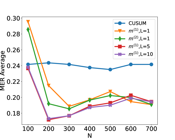
\n ## Line Chart: MER Average vs. N for Different Algorithms ### Overview The image is a line chart comparing the performance of five different algorithms or methods. The performance metric is "MER Average" plotted against a parameter "N". The chart shows how the average MER (likely Mean Error Rate or a similar metric) changes as N increases from 100 to 700 for each method. ### Components/Axes * **X-Axis:** Labeled "N". It has major tick marks at intervals of 100, ranging from 100 to 700. * **Y-Axis:** Labeled "MER Average". It has major tick marks at intervals of 0.02, ranging from 0.18 to 0.30. * **Legend:** Located in the top-right corner of the plot area. It contains five entries, each with a unique color, marker, and label: 1. Blue line with circle markers: `CUSUM` 2. Orange line with downward-pointing triangle markers: `m^{(1)}, L=1` 3. Green line with diamond markers: `m^{(2)}, L=1` 4. Red line with square markers: `m^{(1)}, L=5` 5. Purple line with 'x' markers: `m^{(1)}, L=10` ### Detailed Analysis **Trend Verification & Data Point Extraction (Approximate Values):** 1. **CUSUM (Blue, Circle):** * **Trend:** The line is relatively flat, showing only minor fluctuations. It starts around 0.24, dips slightly around N=500, and ends near its starting value. * **Data Points:** * N=100: ~0.242 * N=200: ~0.244 * N=300: ~0.242 * N=400: ~0.238 * N=500: ~0.235 * N=600: ~0.242 * N=700: ~0.242 2. **m^{(1)}, L=1 (Orange, Downward Triangle):** * **Trend:** Starts very high, drops sharply until N=300, then exhibits a fluctuating pattern with a local peak at N=500 before declining again. * **Data Points:** * N=100: ~0.296 (Highest point on the chart) * N=200: ~0.216 * N=300: ~0.190 * N=400: ~0.198 * N=500: ~0.208 * N=600: ~0.195 * N=700: ~0.192 3. **m^{(2)}, L=1 (Green, Diamond):** * **Trend:** Starts high, drops sharply until N=300, then shows a gradual, slightly fluctuating increase. * **Data Points:** * N=100: ~0.286 * N=200: ~0.192 * N=300: ~0.185 * N=400: ~0.196 * N=500: ~0.202 * N=600: ~0.198 * N=700: ~0.190 4. **m^{(1)}, L=5 (Red, Square):** * **Trend:** Starts moderately high, drops sharply to a minimum at N=200, then shows a steady, gradual increase. * **Data Points:** * N=100: ~0.236 * N=200: ~0.171 (Lowest point on the chart) * N=300: ~0.177 * N=400: ~0.189 * N=500: ~0.192 * N=600: ~0.203 * N=700: ~0.195 5. **m^{(1)}, L=10 (Purple, 'x'):** * **Trend:** Follows a very similar path to the red line (m^{(1)}, L=5), starting at a similar point, dropping to a minimum at N=200, and then gradually increasing, though it remains slightly below the red line for most points after N=300. * **Data Points:** * N=100: ~0.238 * N=200: ~0.173 * N=300: ~0.177 * N=400: ~0.187 * N=500: ~0.190 * N=600: ~0.200 * N=700: ~0.194 ### Key Observations 1. **Initial Performance Gap:** At the smallest N (100), there is a wide spread in performance. The `m^{(1)}, L=1` method has the highest MER (~0.296), while `CUSUM` and the `L=5`/`L=10` variants are clustered around ~0.24. 2. **Convergence at Low N:** All methods except `CUSUM` show a dramatic improvement (decrease in MER) as N increases from 100 to 200 or 300. The lowest overall MER values are achieved around N=200-300. 3. **CUSUM Stability:** The `CUSUM` method is an outlier in its behavior. It shows very little sensitivity to the parameter N, maintaining a nearly constant MER average between ~0.235 and ~0.244 across the entire range. 4. **Post-Convergence Behavior:** After N=300, the methods diverge again. The `m^{(1)}` variants (L=1,5,10) and `m^{(2)}, L=1` show a general trend of slightly increasing MER with N, while `CUSUM` remains flat. 5. **Effect of Parameter L:** For the `m^{(1)}` family, increasing L from 1 to 5 or 10 significantly improves performance (lowers MER) at small N (100-200). At larger N (≥400), the differences between L=5 and L=10 are minimal, and both are generally outperformed by `m^{(2)}, L=1`. ### Interpretation This chart likely compares the performance of different change-point detection or sequential analysis algorithms. "MER Average" is probably a measure of error or detection delay, where lower is better. "N" could represent sample size, sequence length, or a similar parameter. The data suggests a clear trade-off: * **CUSUM** is robust and stable, providing predictable, moderate performance regardless of N. It doesn't excel at any point but also doesn't degrade. * The **`m` methods** (likely referring to some multi-customer or multi-stream variant) are highly sensitive to N. They can achieve significantly lower error rates than CUSUM (especially `m^{(2)}, L=1` and `m^{(1)}, L=5/10` around N=200-300), but their performance deteriorates if N is too small or, to a lesser extent, too large. * The **parameter L** (possibly a window size or memory length) is crucial for the `m^{(1)}` method. A larger L (5 or 10) provides much better initial performance than L=1, suggesting that incorporating more history is beneficial when data is scarce (low N). * The **`m^{(2)}` variant** with L=1 shows a compelling profile: it starts with high error but quickly drops to become one of the best-performing methods for N≥200, often matching or beating the `m^{(1)}` methods with larger L values. **In summary:** The choice of algorithm depends heavily on the expected operating range of N. For a wide, unpredictable range of N, CUSUM offers safety. If N can be controlled or is known to be in the 200-400 range, the `m` methods (particularly `m^{(2)}, L=1` or `m^{(1)}, L=5`) offer superior performance. The chart demonstrates that algorithmic parameters (like L) must be tuned relative to the problem scale (N).