TECHNICAL ASSET FINGERPRINT
500de4a24062dc7e5ef3d073
Click to view fullscreen
Press ESC or click to close
FOUND IN PAPERS
EXPERT: healer-alpha-free VERSION 1
RUNTIME: free/openrouter/healer-alpha
INTEL_VERIFIED
## [Multi-Panel Technical Figure]: Comparison of Easy vs. Difficult Experimental Setups
### Overview
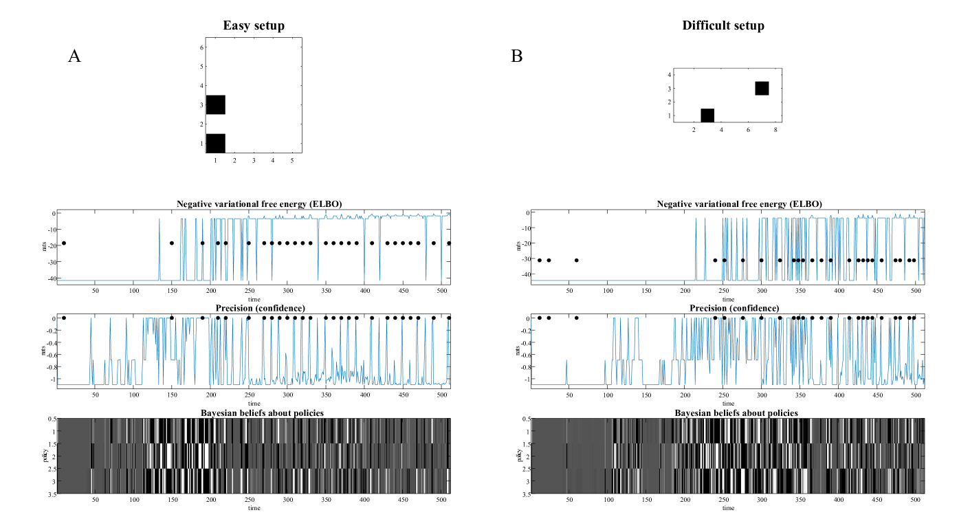
The image is a composite figure containing two main columns, labeled **A** and **B**, which compare results from an "Easy setup" and a "Difficult setup," respectively. Each column contains four plots: a top scatter plot and three time-series plots below it. The figure appears to present data from a computational or machine learning experiment, likely involving Bayesian inference, active inference, or reinforcement learning, tracking metrics like variational free energy (ELBO), precision (confidence), and policy beliefs over time.
### Components/Axes
**Top Row (Scatter Plots):**
* **Plot A (Left):** Titled **"Easy setup"**. It is a 2D scatter plot with an x-axis ranging from 1 to 5 and a y-axis ranging from 1 to 6. Two black square markers are present: one at approximate coordinates **(1, 1)** and another at **(1, 3)**.
* **Plot B (Right):** Titled **"Difficult setup"**. It is a 2D scatter plot with an x-axis ranging from 2 to 8 and a y-axis ranging from 1 to 4. Two black square markers are present: one at approximate coordinates **(3, 1)** and another at **(7, 3)**.
**Time-Series Plots (Both Columns A and B share identical structure):**
1. **Top Time-Series:** Titled **"Negative variational free energy (ELBO)"**.
* **X-axis:** Label is **"time"**, scale from 0 to 500.
* **Y-axis:** Label is **"nats"**, scale from -40 to 0.
* **Data:** A continuous blue line plot with overlaid black circular dots at specific time points.
2. **Middle Time-Series:** Titled **"Precision (confidence)"**.
* **X-axis:** Label is **"time"**, scale from 0 to 500.
* **Y-axis:** Label is **"nats"**, scale from -1 to 0.
* **Data:** A continuous blue line plot with overlaid black circular dots at specific time points.
3. **Bottom Time-Series:** Titled **"Bayesian beliefs about policies"**.
* **X-axis:** Label is **"time"**, scale from 0 to 500.
* **Y-axis:** Label is **"policy"**, scale from 0.5 to 3.5.
* **Data:** A grayscale heatmap or raster plot. The intensity (darkness) represents the probability or belief strength for different discrete policies (y-axis) over time (x-axis). Darker shades indicate higher belief.
### Detailed Analysis
**A. Easy Setup Time-Series Trends:**
* **ELBO:** The blue line starts near -40 nats. Around time=150, it begins to exhibit sharp, frequent upward spikes towards 0 nats, interspersed with returns to lower values. From approximately time=250 onward, the signal oscillates rapidly between high (near 0) and low values, with the black dots appearing predominantly during the high-value phases.
* **Precision:** The blue line shows a pattern of frequent, sharp drops from near 0 nats down to -1 nats, especially between time=50-150. After time=150, the drops become more frequent and are often followed by rapid recoveries. The black dots are clustered during periods where the precision is sustained near 0.
* **Bayesian Beliefs:** The heatmap shows distinct vertical bands. Initially (time 0-50), belief is concentrated on a single policy (around y=1.5). Over time, belief shifts and becomes distributed across multiple policies (y=1 to 3), with clear, rapid transitions between dominant policies, visualized as sharp changes from light to dark vertical stripes.
**B. Difficult Setup Time-Series Trends:**
* **ELBO:** Similar initial low value. The first major upward spike occurs later, around time=220. The subsequent oscillations between high and low values appear more erratic and less densely packed than in the Easy setup. The black dots are scattered, with a notable cluster after time=300.
* **Precision:** Shows a very sparse pattern of drops to -1 nats before time=100. After time=100, it enters a phase of extremely frequent and deep oscillations between 0 and -1 nats, which continues for the remainder of the timeline. The black dots are sparse early on but become densely clustered after time=300, aligning with the period of intense oscillation.
* **Bayesian Beliefs:** The heatmap shows a more gradual and complex evolution of beliefs. There is less clear, sustained dominance of a single policy compared to the Easy setup. The transitions between policy beliefs appear more frequent and noisier, with many policies showing intermediate (gray) levels of belief simultaneously.
### Key Observations
1. **Temporal Onset:** The "Difficult setup" shows a delayed onset of significant activity (spikes in ELBO, drops in Precision) compared to the "Easy setup."
2. **Signal Character:** The "Easy setup" time-series, particularly after time=250, show more regular, high-frequency oscillations. The "Difficult setup" signals appear more chaotic and less periodic.
3. **Dot Alignment:** In both setups, the black dots (likely indicating decision points, observations, or actions) tend to cluster during periods of high ELBO (near 0 nats) and high Precision (near 0 nats). This correlation is more pronounced in the latter half of the timelines.
4. **Policy Belief Dynamics:** The "Easy setup" exhibits clearer, more decisive shifts in policy belief (sharp black/white transitions). The "Difficult setup" shows more ambiguous, distributed beliefs (more gray areas) and faster, less stable switching.
### Interpretation
This figure contrasts the performance of an agent or model under two conditions of environmental or task difficulty.
* **What the data suggests:** The "Easy setup" allows the system to achieve high ELBO (good model fit/evidence accumulation) and high precision (confidence) more quickly and maintain it with regular, confident updates (dots). Its policy beliefs are decisive. The "Difficult setup" delays this convergence. The system struggles initially, then enters a state of high but unstable confidence (frequent precision drops) and erratic model evidence (ELBO spikes). Its policy beliefs remain uncertain and fluctuate rapidly, suggesting difficulty in identifying a stable, optimal strategy.
* **Relationship between elements:** The top scatter plots likely define the experimental conditions (e.g., locations of targets or stimuli in a 2D space). The time-series show the internal state of the agent responding to those conditions. High ELBO and Precision are prerequisites for confident policy selection, as seen by the dot clustering. The Bayesian beliefs plot is the direct output of this inference process.
* **Notable anomalies/trends:** The most striking trend is the **phase transition** in both setups around a specific time (≈150 for Easy, ≈220 for Difficult), where the system shifts from a low-activity state to a high-activity, oscillatory state. The "Difficult setup" never achieves the same regularity or stability as the "Easy setup," indicating a fundamental limit in its ability to resolve the more challenging task configuration. The persistent oscillations in Precision in the Difficult case may reflect a system constantly testing and rejecting hypotheses.
DECODING INTELLIGENCE...