## Neural Network Diagram: Base Model vs. Sparse Model
### Overview
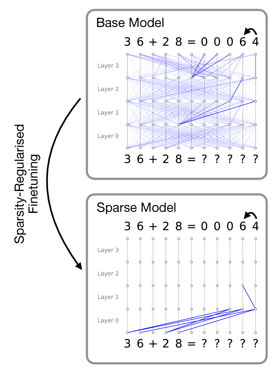
The image presents two diagrams illustrating the architecture and connectivity of a "Base Model" and a "Sparse Model" neural network. Both models are depicted as solving the arithmetic problem "36 + 28". The Base Model shows dense connections between layers, while the Sparse Model shows significantly fewer connections, achieved through sparsity-regularized fine-tuning. An arrow indicates the transformation from the Base Model to the Sparse Model.
### Components/Axes
* **Titles:** "Base Model" (top), "Sparse Model" (bottom)
* **Layers:** Both models have layers labeled "Layer 0", "Layer 1", "Layer 2", and "Layer 3". These labels are positioned vertically to the left of each model's network diagram.
* **Nodes:** Each layer consists of a series of nodes, represented as small circles.
* **Connections:** The connections between nodes in adjacent layers are represented by blue lines. The Base Model has many connections, while the Sparse Model has very few.
* **Input/Output:** Both models show the input "36 + 28 =" at the bottom. The Base Model shows the output "?????", while the Sparse Model shows the output "?????".
* **Solution:** Above the "Layer 3" layer, both models show the solution "36 + 28 = 0 0 0 6 4". An arrow indicates the direction of the solution.
* **Transformation Arrow:** A curved arrow on the left side of the image indicates the transformation from the Base Model to the Sparse Model, labeled "Sparsity-Regularised Finetuning".
### Detailed Analysis
**Base Model:**
* **Input:** "36 + 28 = ?????".
* **Layer 0:** Seven nodes.
* **Layer 1:** Seven nodes.
* **Layer 2:** Seven nodes.
* **Layer 3:** Seven nodes.
* **Output:** "36 + 28 = 0 0 0 6 4".
* **Connections:** Dense connections between all nodes in adjacent layers. Each node in a layer is connected to almost every node in the next layer.
**Sparse Model:**
* **Input:** "36 + 28 = ?????".
* **Layer 0:** Seven nodes.
* **Layer 1:** Seven nodes.
* **Layer 2:** Seven nodes.
* **Layer 3:** Seven nodes.
* **Output:** "36 + 28 = 0 0 0 6 4".
* **Connections:** Sparse connections between nodes. Only a few nodes in each layer are connected to nodes in the next layer. The connections are concentrated in the lower layers (Layer 0 and Layer 1).
**Transformation:**
* The arrow labeled "Sparsity-Regularised Finetuning" indicates that the Sparse Model is derived from the Base Model through a process of sparsity regularization and fine-tuning.
### Key Observations
* The Base Model has a fully connected architecture, while the Sparse Model has a highly sparse architecture.
* The sparsity in the Sparse Model is achieved through sparsity-regularized fine-tuning.
* Both models are designed to solve the same arithmetic problem.
* The Sparse Model retains the ability to solve the problem despite having significantly fewer connections.
### Interpretation
The diagrams illustrate the concept of sparsity in neural networks. Sparsity regularization is a technique used to reduce the number of connections in a neural network, which can lead to several benefits, including:
* **Reduced computational cost:** Fewer connections mean fewer parameters to train and fewer operations to perform during inference.
* **Improved generalization:** Sparse models are less likely to overfit the training data, which can lead to better performance on unseen data.
* **Increased interpretability:** Sparse models are often easier to interpret because the connections that remain are more likely to be important.
The image demonstrates that it is possible to create a sparse model that performs as well as a dense model, while also enjoying the benefits of sparsity. The "Sparsity-Regularised Finetuning" process is crucial for achieving this result. The fact that both models arrive at the same solution "0 0 0 6 4" suggests that the sparse model has successfully retained the essential information needed to solve the problem.