## Diagram: Effect of Sparsity-Regularised Finetuning on a Neural Network
### Overview
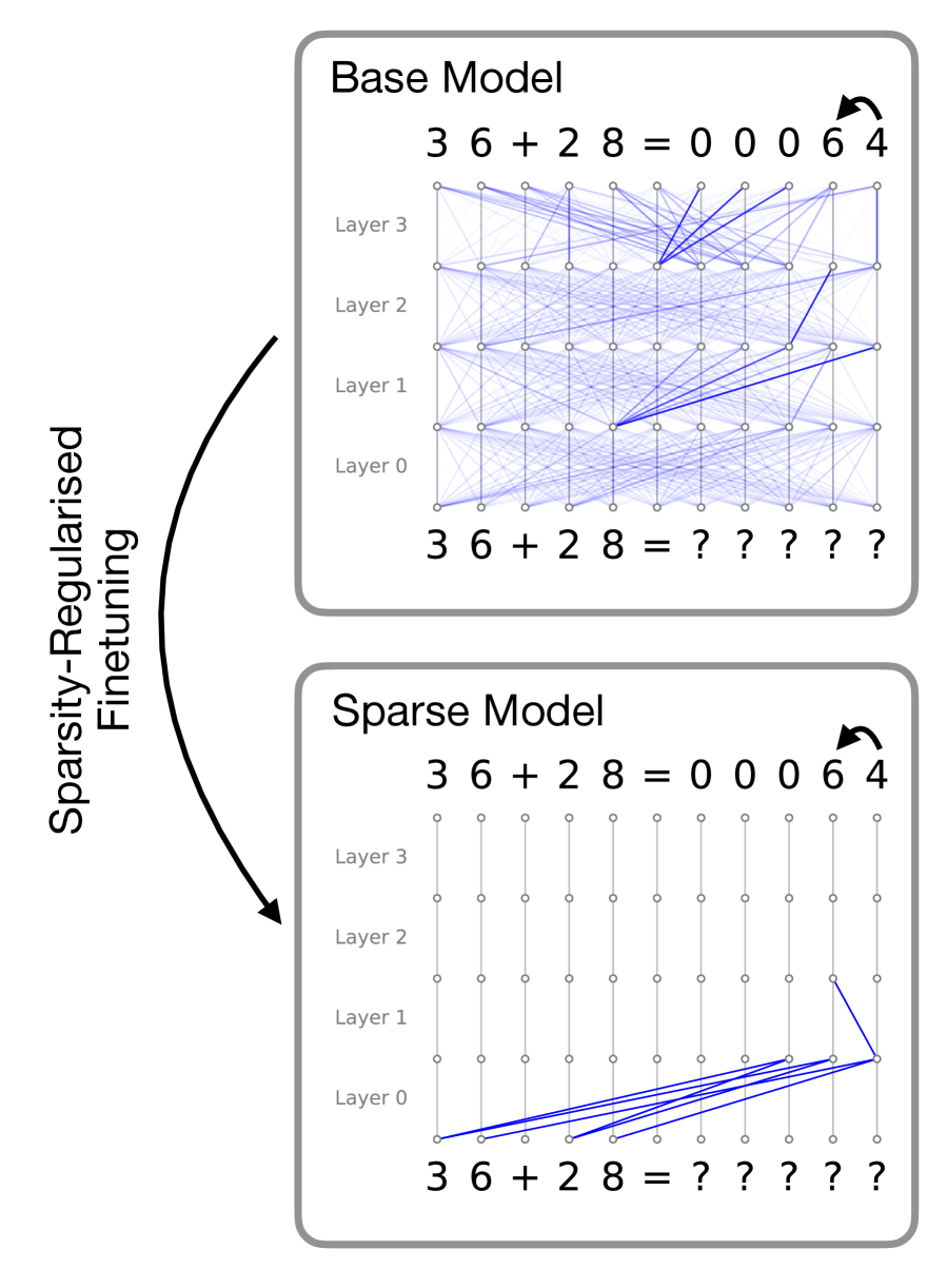
This image is a technical diagram illustrating the structural changes within a neural network (likely a Transformer model) before and after a process called "Sparsity-Regularised Finetuning." It compares a "Base Model" with dense, complex internal connections to a "Sparse Model" with highly pruned, efficient connections, both performing the same mathematical addition task.
*Language Declaration:* All text in this image is in English.
### Components/Axes
The image is divided into three main spatial regions:
1. **Left Margin (Process Indicator):** Contains vertical text and a directional arrow indicating the transformation process.
2. **Top Panel (Base Model):** A bounded box showing the initial state of the neural network.
3. **Bottom Panel (Sparse Model):** A bounded box showing the final state of the neural network.
**Axes & Grid System (Present in both panels):**
* **X-Axis (Implicit - Sequence Position):** Represents the sequence of tokens (characters) in the input and output strings. There are 11 columns corresponding to the 11 characters in the equation.
* **Y-Axis (Network Depth):** Labeled on the left side of the grid from bottom to top: `Layer 0`, `Layer 1`, `Layer 2`, `Layer 3`.
* **Nodes:** Small circles arranged in an 11x5 grid (Input level + 4 hidden layers).
* **Edges (Lines):** Represent attention weights or information flow between nodes.
* *Blue lines:* Active connections (thicker/darker indicates stronger weight).
* *Gray vertical lines:* Residual stream or pass-through connections within the same token column.
### Content Details
#### 1. Left Margin (Process Indicator)
* **Text:** "Sparsity-Regularised Finetuning" (Oriented vertically, reading from bottom to top).
* **Graphic:** A thick, black, curved arrow originates beside the top panel and points downward to the bottom panel, indicating that the Base Model is transformed into the Sparse Model via this finetuning method.
#### 2. Top Panel: Base Model
* **Header:** "Base Model" (Top-left).
* **Output Sequence (Top row):** `3 6 + 2 8 = 0 0 0 6 4`
* *Annotation:* A small, curved black arrow points from the `6` to the `4` at the end of the sequence. This indicates the specific step being visualized: the autoregressive prediction of the final token ('4') given the preceding context.
* **Input Sequence (Bottom row):** `3 6 + 2 8 = ? ? ? ? ?`
* **Visual Trend (Network Connections):** The grid is filled with a dense, chaotic web of light blue lines connecting nodes across different columns and layers.
* **Specific Routing:** While dense, darker blue lines show a concentration of information flowing from various nodes in Layers 0, 1, and 2 towards the nodes in the final two columns of Layers 2 and 3, ultimately converging to predict the final '4'.
#### 3. Bottom Panel: Sparse Model
* **Header:** "Sparse Model" (Top-left).
* **Output Sequence (Top row):** `3 6 + 2 8 = 0 0 0 6 4`
* *Annotation:* Identical curved black arrow pointing from `6` to `4`.
* **Input Sequence (Bottom row):** `3 6 + 2 8 = ? ? ? ? ?`
* **Visual Trend (Network Connections):** The dense web is entirely gone. The vast majority of nodes only connect vertically to themselves via thin gray lines. Cross-column communication (blue lines) is drastically reduced to a single, highly specific pathway.
* **Specific Routing:**
* At the input level (below Layer 0), dark blue lines originate *only* from the numerical operands: `3`, `6`, `2`, and `8`.
* These four lines converge directly into a single node at **Layer 0** in the second-to-last column (the column corresponding to the output '6').
* From that node in Layer 0, a single dark blue line travels up and right to a node in **Layer 1** in the final column.
* From Layer 1 upwards in the final column, the information flows vertically to output the '4'.
### Key Observations
* **Task Identification:** The model is performing integer addition: 36 + 28 = 64. The output is padded with leading zeros (00064).
* **Identical Outputs:** Both the Base Model and the Sparse Model successfully predict the correct final digit ('4'), proving that the pruning process did not destroy the model's capability to perform the task.
* **Drastic Reduction in Complexity:** The Base Model uses almost all available attention pathways (dense cross-talk). The Sparse Model isolates the exact mathematical "circuit" required, ignoring irrelevant tokens like the space, `+`, and `=` signs during this specific prediction step.
### Interpretation
This diagram is a powerful visualization of **Mechanistic Interpretability** and the effects of **Sparsity**.
1. **Algorithmic Clarity:** In standard large language models (the Base Model), information routing is highly distributed and polysemantic, making it nearly impossible for humans to understand *how* the model arrives at an answer. By applying Sparsity-Regularised Finetuning, the model is penalized for using unnecessary connections. It is forced to find the most efficient, minimal sub-network (a "circuit") to solve the problem.
2. **Reading the Circuit:** The Sparse Model reveals the underlying algorithm the network has learned. To predict the final digit of the sum of 36 and 28, the model *only* needs to look at the digits themselves (3, 6, 2, 8). It routes these specific digits into a calculation node early in the network (Layer 0/1), computes the result, and passes it up the residual stream to the output. It completely ignores the operator (`+`) and the equals sign (`=`), likely because the context of the task is already embedded in the residual stream, or those tokens are unnecessary for the raw calculation of the final digit.
3. **Practical Implications:** A model that looks like the bottom panel is highly desirable. It is interpretable (we can prove how it does math), it is less prone to hallucination based on irrelevant context (because those attention heads are turned off), and if implemented at the hardware level, sparse matrices require significantly less compute and memory than dense matrices.