## Diagram: Neural Network Sparsity Regularization Comparison
### Overview
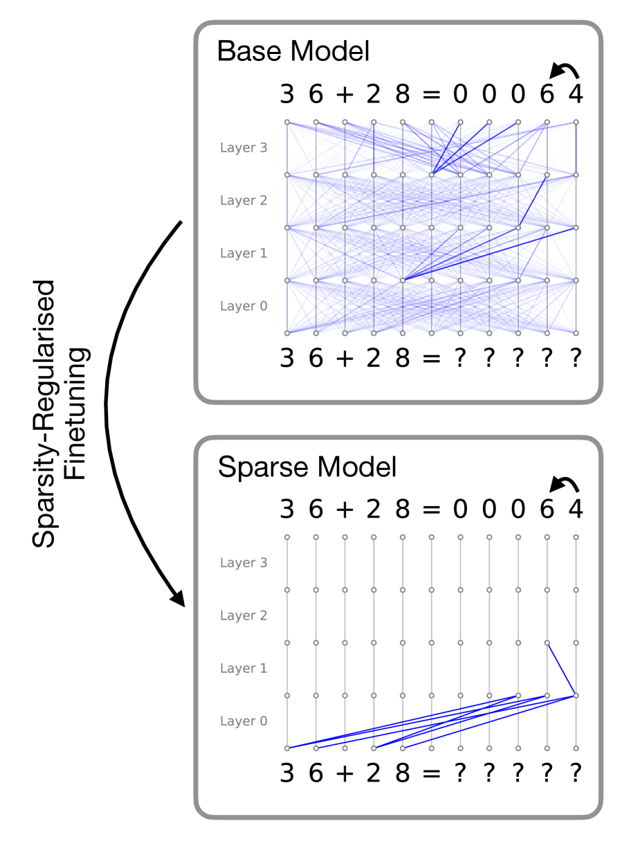
The image is a technical diagram comparing the internal connectivity of two neural network models—a "Base Model" and a "Sparse Model"—before and after a process labeled "Sparsity-Regularised Finetuning." It visually demonstrates how the finetuning process drastically reduces the number of active connections (weights) within the network while maintaining the same input-output function for a simple arithmetic task.
### Components/Axes
The diagram is divided into two primary rectangular panels, stacked vertically, with a large curved arrow connecting them on the left.
1. **Top Panel: "Base Model"**
* **Title:** "Base Model" (top-left corner of the panel).
* **Input Sequence (Bottom):** `3 6 + 2 8 = ? ? ? ? ?`
* **Output Sequence (Top):** `3 6 + 2 8 = 0 0 0 6 4`
* **Network Structure:** A grid of nodes representing neurons, organized into four horizontal rows labeled from bottom to top: "Layer 0", "Layer 1", "Layer 2", "Layer 3".
* **Connections:** A dense web of light blue lines connects nodes between adjacent layers. Several connections are highlighted in a darker, more prominent blue, indicating stronger or more significant weights. The connections are dense and distributed across all layers.
2. **Bottom Panel: "Sparse Model"**
* **Title:** "Sparse Model" (top-left corner of the panel).
* **Input Sequence (Bottom):** `3 6 + 2 8 = ? ? ? ? ?`
* **Output Sequence (Top):** `3 6 + 2 8 = 0 0 0 6 4`
* **Network Structure:** Identical grid layout and layer labels ("Layer 0" to "Layer 3") as the Base Model.
* **Connections:** The vast majority of connections are absent. Only a small cluster of dark blue lines remains, almost exclusively connecting nodes from the input sequence directly to nodes in "Layer 0". A single, isolated connection is visible between Layer 1 and Layer 2 on the far right.
3. **Connecting Element:**
* A large, black, curved arrow points from the "Base Model" panel down to the "Sparse Model" panel.
* **Label:** The text "Sparsity-Regularised Finetuning" is written vertically along the left side of this arrow.
### Detailed Analysis
* **Task:** Both models are performing the same arithmetic task: calculating `36 + 28`. The correct answer, `00064` (likely representing a 5-digit output format), is shown as the target output for both.
* **Connectivity Trend - Base Model:** The Base Model exhibits a "dense" or fully-connected-like architecture. Information flows through a complex, distributed network of connections across all four layers. The darker blue lines suggest certain pathways are more active or important for this specific computation.
* **Connectivity Trend - Sparse Model:** The Sparse Model exhibits extreme sparsity. The finetuning process has pruned nearly all connections. The remaining active pathways are highly localized:
* **Primary Cluster:** A fan of dark blue connections originates from the nodes representing the digits `3`, `6`, `+`, `2`, `8` in the input line and converges onto a subset of nodes in **Layer 0**. This suggests the model has learned to perform the core computation using direct, early-layer feature extraction.
* **Isolated Connection:** One dark blue line connects a node in Layer 1 to a node in Layer 2 on the far right side of the grid. This may represent a minimal residual pathway for propagating the result.
* **Output Consistency:** Crucially, the output `0 0 0 6 4` is identical in both models, indicating that the sparse model retains the functional capability of the dense base model for this task.
### Key Observations
1. **Dramatic Pruning:** The "Sparsity-Regularised Finetuning" process removes the vast majority of neural connections, transforming a dense network into a highly sparse one.
2. **Functional Preservation:** Despite the massive reduction in parameters (connections), the sparse model produces the exact same correct output for the given input.
3. **Localization of Computation:** The remaining computation in the sparse model is heavily concentrated in the first layer (Layer 0), with direct connections from the input. This implies the essential logic for solving `36 + 28` can be encoded with very few, direct transformations.
4. **Architectural Insight:** The diagram suggests that for this specific, simple algorithmic task, a dense network is over-parameterized. The true computational "circuit" required is small and can be isolated via sparsity-inducing techniques.
### Interpretation
This diagram is a powerful visual argument for the efficacy of **sparsity regularization** in neural network training. It demonstrates that:
* **Efficiency through Sparsity:** Large, dense models contain significant redundancy. Techniques like sparsity regularization can identify and preserve only the essential sub-network (a "winning ticket") needed for a specific task, leading to models that are potentially much smaller and faster.
* **Mechanistic Understanding:** The process acts as a form of "circuit discovery." By pruning away unused connections, it reveals the minimal computational graph the network uses to solve the problem. Here, the core arithmetic appears to be handled by direct input-to-first-layer mappings.
* **Generalization vs. Specialization:** While shown for a simple task, the principle raises questions about how such sparse sub-networks might generalize to more complex problems. The diagram highlights a trade-off: the sparse model is highly efficient for this task but may lack the distributed representation that could be beneficial for broader reasoning.
In essence, the image moves beyond showing *that* sparsity works to illustrating *how* it works—by surgically removing non-essential pathways and leaving behind a lean, functional core.