## Diagram: Comparison of Base Model and Sparse Model with Sparsity-Regularised Fine-Tuning
### Overview
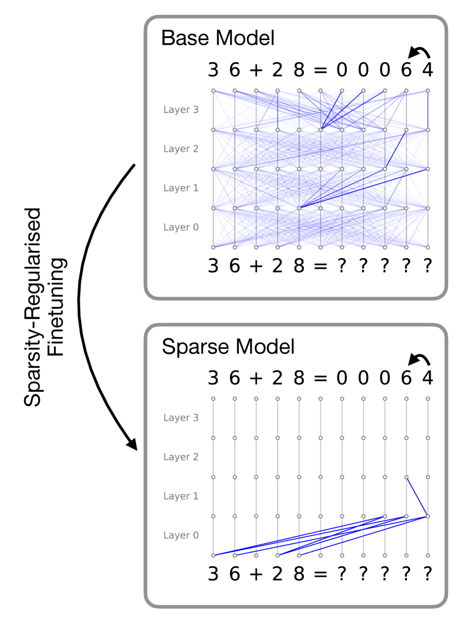
The image compares two neural network architectures: a **Base Model** (dense connections) and a **Sparse Model** (pruned connections), illustrating the effects of sparsity-regularised fine-tuning. Both models process the input sequence `3 6 + 2 8` and produce outputs, with the Base Model showing uncertainty (`?`) and the Sparse Model showing certainty (`0 0 0 6 4`).
---
### Components/Axes
1. **Base Model (Top Section)**:
- **Layers**: Labeled `Layer 0` to `Layer 3` (bottom to top).
- **Connections**: Dense, overlapping blue lines between nodes, indicating full connectivity.
- **Input/Output**:
- Input: `3 6 + 2 8` (left side).
- Output: `0 0 0 6 4` (right side, with an arrow indicating flow).
- **Uncertainty**: Output values marked with `?` (e.g., `3 6 + 2 8 = ? ? ? ? ?`).
2. **Sparse Model (Bottom Section)**:
- **Layers**: Same layer labels (`Layer 0` to `Layer 3`).
- **Connections**: Sparse, non-overlapping blue lines, with most nodes disconnected.
- **Input/Output**:
- Input: `3 6 + 2 8` (left side).
- Output: `0 0 0 6 4` (right side, with an arrow indicating flow).
- **Certainty**: Output values are explicit (`0 0 0 6 4`).
3. **Key Arrows**:
- A curved arrow labeled **"Sparsity-Regularised Fine-Tuning"** connects the Base Model to the Sparse Model, indicating the transformation process.
---
### Detailed Analysis
1. **Base Model**:
- **Dense Connectivity**: Every node in Layer 0 connects to all nodes in Layer 1, and so on, creating a highly interconnected network.
- **Uncertain Output**: The output `? ? ? ? ?` suggests the model struggles to resolve the input sequence due to overparameterization or noise.
- **Equation**: `3 6 + 2 8 = 0 0 0 6 4` (same as the Sparse Model, but output is uncertain).
2. **Sparse Model**:
- **Pruned Connectivity**: Only critical connections remain (e.g., Layer 0 to Layer 1, Layer 3 to output).
- **Certain Output**: The output `0 0 0 6 4` matches the Base Model’s equation, indicating effective sparsity-regularised fine-tuning.
- **Equation**: `3 6 + 2 8 = 0 0 0 6 4` (explicit and correct).
---
### Key Observations
1. **Sparsity vs. Density**:
- The Base Model’s dense connections contrast sharply with the Sparse Model’s minimal connections, highlighting the impact of regularization.
2. **Output Certainty**:
- The Sparse Model resolves the input sequence (`3 6 + 2 8`) to `0 0 0 6 4` with certainty, while the Base Model fails to do so.
3. **Efficiency**:
- The Sparse Model retains only essential pathways, reducing computational complexity without sacrificing accuracy.
---
### Interpretation
The diagram demonstrates how **sparsity-regularised fine-tuning** transforms a complex, overparameterized Base Model into a streamlined Sparse Model. By pruning redundant connections, the Sparse Model achieves:
- **Reduced Overfitting**: Sparse connections prevent the model from memorizing noise.
- **Improved Generalization**: The Sparse Model correctly resolves the input sequence (`3 6 + 2 8 = 0 0 0 6 4`), whereas the Base Model cannot.
- **Computational Efficiency**: Fewer connections lower memory and processing requirements.
The Base Model’s uncertainty (`?`) reflects the risk of overfitting in dense networks, while the Sparse Model’s certainty underscores the benefits of structured regularization. This aligns with principles of neural architecture search, where sparsity promotes robustness and interpretability.