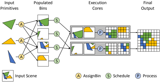
## Diagram: Geometric Primitive Processing Pipeline ### Overview This diagram illustrates a multi-stage parallel processing pipeline for geometric primitives, transforming them from individual shapes into a combined rasterized output. The process involves assigning input primitives to spatial bins, scheduling these bins to parallel execution cores, processing the primitives within each core, and finally aggregating the results into a single output grid. ### Components/Axes The diagram is structured into four main conceptual stages, labeled horizontally from left to right: 1. **Input Primitives**: The initial geometric shapes. 2. **Populated Bins**: Collections of primitives grouped into logical units. 3. **Execution Cores**: Parallel processing units. 4. **Final Output**: The aggregated, rasterized result. **Legend (located at the bottom of the diagram):** * **Input Scene**: Represented by a white square containing an overlapping green irregular quadrilateral, a yellow trapezoid, and a blue irregular triangle. This symbol is used to depict the contents of the "Populated Bins" and the inputs to the "Execution Cores". * **(A) AssignBin**: Represented by a yellow circular node with the letter 'A'. This component is responsible for distributing input primitives to bins. * **(S) Schedule**: Represented by a green circular node with the letter 'S'. This component is responsible for assigning populated bins to execution cores. * **(P) Process**: Represented by a blue circular node with the letter 'P'. This component performs the actual processing (e.g., rasterization) of primitives within an execution core. ### Detailed Analysis **1. Input Primitives (Leftmost Column):** Three distinct geometric primitives are shown vertically: * **Top**: A green irregular quadrilateral/pentagon. * **Middle**: A yellow trapezoid. * **Bottom**: A blue irregular triangle/quadrilateral. **2. AssignBin (A) Nodes:** Three yellow circular 'A' nodes are positioned to the right of the input primitives. Each 'A' node receives an arrow from one input primitive: * The top 'A' node receives input from the green primitive. * The middle 'A' node receives input from the yellow primitive. * The bottom 'A' node receives input from the blue primitive. Each 'A' node has multiple outgoing arrows connecting to the "Populated Bins", indicating that a single primitive can be assigned to multiple bins. **3. Populated Bins (Second Column from Left):** Four white square bins are arranged vertically. Each bin contains a combination of the input primitives, representing an "Input Scene" as per the legend. * **Bin 1 (Top)**: Contains the majority of the green primitive and a small portion of the blue primitive. It receives input from the top 'A' (green primitive) and the bottom 'A' (blue primitive). * **Bin 2**: Contains a small portion of the green primitive and a small portion of the yellow primitive. It receives input from the top 'A' (green primitive) and the middle 'A' (yellow primitive). * **Bin 3**: Contains the majority of the blue primitive and a small portion of the yellow primitive. It receives input from the middle 'A' (yellow primitive) and the bottom 'A' (blue primitive). * **Bin 4 (Bottom)**: Contains the majority of the yellow primitive. It receives input from the middle 'A' (yellow primitive). Each bin has an outgoing arrow leading to a "Schedule (S)" node. **4. Schedule (S) Nodes:** Four green circular 'S' nodes are positioned to the right of the populated bins. Each 'S' node receives an arrow from one populated bin. These nodes then direct their output to the "Execution Cores" with cross-connections: * The top 'S' node (from Bin 1) directs its output to the top "Execution Core" (left input scene). * The second 'S' node (from Bin 2) directs its output to the top "Execution Core" (right input scene). * The third 'S' node (from Bin 3) directs its output to the bottom "Execution Core" (left input scene). * The bottom 'S' node (from Bin 4) directs its output to the bottom "Execution Core" (right input scene). **5. Execution Cores (Third Column from Left):** Two grey rectangular units represent two parallel execution cores. Each core processes two input scenes and produces two corresponding 4x4 pixel grids. * **Top Execution Core**: * **Input Scenes**: * Left: Contains the green primitive (mostly) and a small part of the blue primitive (from Bin 1). * Right: Contains a small part of the green primitive and a small part of the yellow primitive (from Bin 2). * **Process (P) Node**: A blue circular 'P' node is centrally located within the core, indicating the processing step. * **Output Grids (4x4 pixels)**: * Left Grid (from left input scene): * Row 1: 1 blue pixel (bottom-left), 3 white pixels. * Row 2: 4 green pixels. * Row 3: 4 green pixels. * Row 4: 4 green pixels. * Right Grid (from right input scene): * Row 1: 4 white pixels. * Row 2: 4 white pixels. * Row 3: 1 yellow pixel (bottom-left), 3 white pixels. * Row 4: 1 green pixel (bottom-left), 3 white pixels. * **Bottom Execution Core**: * **Input Scenes**: * Left: Contains the blue primitive (mostly) and a small part of the yellow primitive (from Bin 3). * Right: Contains the yellow primitive (mostly) (from Bin 4). * **Process (P) Node**: A blue circular 'P' node is centrally located within the core. * **Output Grids (4x4 pixels)**: * Left Grid (from left input scene): * Row 1: 4 white pixels. * Row 2: 4 white pixels. * Row 3: 1 yellow pixel (bottom-left), 3 white pixels. * Row 4: 4 blue pixels. * Right Grid (from right input scene): * Row 1: 4 white pixels. * Row 2: 4 white pixels. * Row 3: 4 white pixels. * Row 4: 4 yellow pixels. **6. Final Output (Rightmost Column):** A single 8x8 pixel grid is shown, representing the combined output from both execution cores. The top 4x8 section is derived from the top core's outputs (left 4x4 and right 4x4 grids concatenated horizontally), and the bottom 4x8 section is derived from the bottom core's outputs. The combined 8x8 grid is as follows (reading left to right, top to bottom): * **Row 1**: Blue (1), White (7) * **Row 2**: Green (4), White (4) * **Row 3**: Green (4), Yellow (1), White (3) * **Row 4**: Green (5), White (3) * **Row 5**: White (8) * **Row 6**: White (8) * **Row 7**: Yellow (1), White (7) * **Row 8**: Blue (4), Yellow (4) ### Key Observations * **Parallelism**: The diagram clearly depicts parallel processing at multiple stages, with multiple bins and two execution cores operating concurrently. * **Spatial Partitioning/Binning**: Input primitives are distributed into "bins," which appear to represent spatial regions or subsets of a larger scene. A single primitive can contribute to multiple bins if it overlaps multiple regions. * **Scheduling**: The "Schedule" step implies a mechanism for distributing workload (bins) efficiently among available "Execution Cores". * **Rasterization**: The "Process" step within the execution cores transforms vector-like geometric primitives into a rasterized (pixel-based) representation. * **Color Consistency**: The colors (green, yellow, blue) consistently represent the same underlying primitive throughout the entire pipeline, from input shapes to individual pixels in the final output. * **Aggregation**: The final output is a composite image formed by combining the rasterized results from the individual execution cores. ### Interpretation This diagram illustrates a common architecture for processing complex geometric scenes, particularly relevant in computer graphics rendering, simulation, or spatial data analysis. The data flow suggests the following: 1. **Decomposition**: A complex scene (implied by the "Input Scene" legend and the multiple primitives) is decomposed into smaller, manageable sub-regions or "bins" by the "AssignBin" function. This allows for localized processing. The fact that a single primitive can be assigned to multiple bins indicates that bins likely represent spatial tiles, and primitives are assigned to all tiles they intersect. 2. **Load Balancing/Resource Allocation**: The "Schedule" function acts as a dispatcher, distributing these populated bins to available "Execution Cores". This step is crucial for optimizing performance in a parallel system, ensuring cores are utilized effectively. 3. **Parallel Processing**: The "Execution Cores" perform the core computational work in parallel. Each core takes a subset of the scene (two bins in this example), processes the geometric primitives within those bins (e.g., rasterizing them into pixels), and generates a partial output. 4. **Reconstruction**: The "Final Output" stage demonstrates the reassembly of these partial, rasterized results from the parallel cores into a complete, coherent image. The pipeline effectively demonstrates how a large computational task (processing a scene with multiple geometric primitives) can be broken down, distributed, processed in parallel, and then reassembled, leading to potentially significant performance gains over a purely sequential approach. The consistent use of color helps to visually trace the contribution of each initial primitive through the various stages of transformation and aggregation.