## Diagram: Parallel Processing Pipeline for Geometric Primitives
### Overview
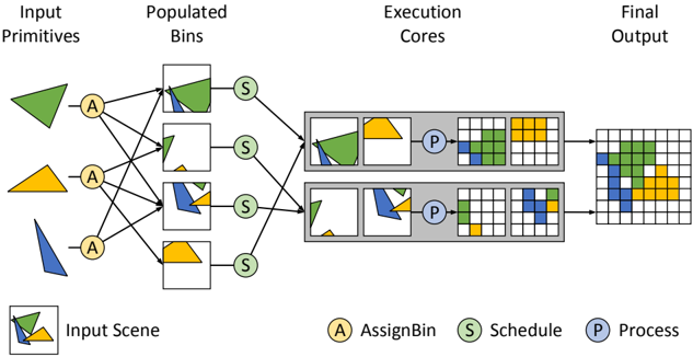
The image is a technical flowchart illustrating a parallel processing pipeline for rendering or computing geometric shapes. It depicts a left-to-right workflow where input shapes are distributed, scheduled, processed in parallel cores, and combined into a final output grid. The diagram uses color-coded shapes (green, yellow, blue triangles) and labeled circular nodes to represent different stages of the process.
### Components/Axes
The diagram is organized into four sequential columns, with a legend and an "Input Scene" reference at the bottom.
**Columns (from left to right):**
1. **Input Primitives:** Contains three distinct geometric shapes:
* A green triangle (top).
* A yellow triangle (middle).
* A blue triangle (bottom).
2. **Populated Bins:** Contains four square bins, each holding a different combination of the input shapes.
* Bin 1 (top): Contains the green triangle and a portion of the blue triangle.
* Bin 2: Contains a small green triangle and a small blue triangle.
* Bin 3: Contains a blue triangle and a small yellow triangle.
* Bin 4 (bottom): Contains the yellow triangle.
3. **Execution Cores:** Contains two parallel processing units (gray rectangles), each with an internal workflow.
* Each core receives input from two of the "Populated Bins" via "Schedule" nodes.
* Inside each core: Input shapes -> A "Process" (P) node -> Intermediate grid representations.
4. **Final Output:** A single, larger grid that combines the processed results from both Execution Cores into one composite image.
**Legend (Bottom Center):**
* **A** (Yellow circle): AssignBin
* **S** (Green circle): Schedule
* **P** (Blue circle): Process
**Input Scene (Bottom Left):**
* A small box showing a composite of the three input triangles (green, yellow, blue) overlapping, labeled "Input Scene."
### Detailed Analysis
**Flow and Connections:**
1. **Assignment Phase:** Each of the three "Input Primitives" connects to a yellow **AssignBin (A)** node. Lines from these 'A' nodes distribute the shapes into the four "Populated Bins." The connections are many-to-many; for example, the green triangle is assigned to the top two bins.
2. **Scheduling Phase:** Each of the four "Populated Bins" connects to a green **Schedule (S)** node. These 'S' nodes then route the bins to one of the two "Execution Cores."
* The top two bins (containing primarily green/blue shapes) are scheduled to the **top Execution Core**.
* The bottom two bins (containing primarily blue/yellow shapes) are scheduled to the **bottom Execution Core**.
3. **Processing Phase:** Within each "Execution Core":
* The scheduled shapes are processed by a blue **Process (P)** node.
* The 'P' node transforms the vector shapes into a pixelated or rasterized grid format. The intermediate grids show the shapes represented as colored blocks (green, yellow, blue) on a white grid.
4. **Output Combination:** The final grid outputs from both Execution Cores are merged to create the single "Final Output" grid. This grid shows all three colored shapes (green, yellow, blue) represented as blocks in their correct relative positions.
**Spatial Grounding:**
* The **legend** is positioned at the bottom center of the entire diagram.
* The **"Input Scene"** reference is in the bottom-left corner.
* The **"Execution Cores"** are stacked vertically in the center-right of the diagram.
* The **"Final Output"** grid is positioned on the far right, centered vertically.
### Key Observations
* **Parallelism:** The core concept is parallel processing. The workload (the four bins) is split between two independent execution cores to speed up computation.
* **Data Distribution:** The initial "AssignBin" stage is responsible for breaking down the input scene into manageable chunks (bins) that can be processed in parallel.
* **Transformation:** The pipeline shows a clear transformation from vector-based "Input Primitives" to rasterized "Final Output" via the "Process" stage.
* **Color Consistency:** The colors of the shapes (green, yellow, blue) are maintained consistently throughout the entire pipeline, from input to final output, allowing for clear tracking.
### Interpretation
This diagram most likely illustrates a **parallel graphics rendering pipeline** or a **computational geometry processing system**. The "Input Primitives" are vector graphics. The "AssignBin" stage performs spatial partitioning or task decomposition, grouping parts of the scene into bins. The "Schedule" stage load-balances these bins across available processing units ("Execution Cores"). The "Process" stage within each core performs the actual rasterization or computation, converting vectors to pixels. Finally, the partial results are composited into the complete "Final Output" image.
The key takeaway is the demonstration of how a complex scene can be efficiently rendered or computed by breaking it into independent tasks, processing them in parallel, and combining the results. This is a fundamental pattern in high-performance computing and real-time graphics. The diagram effectively communicates the flow of data and the separation of concerns (assignment, scheduling, processing) within such a system.