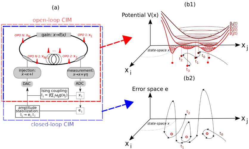
## Diagram: Open-loop and Closed-loop CIM with Potential and Error Space Visualizations ### Overview The image presents a schematic diagram of both open-loop and closed-loop Coherent Ising Machines (CIMs), accompanied by visualizations of the potential landscape and error space associated with the system's dynamics. The diagram is divided into three main sections: (a) showing the CIM configurations, (b1) illustrating the potential V(x), and (b2) illustrating the error space e. ### Components/Axes #### Section (a): CIM Configurations * **Title:** (a) * **Sub-title:** open-loop CIM (enclosed in a dashed red box) * **Sub-title:** closed-loop CIM (enclosed in a dashed blue box) * **Components within the Open-loop CIM:** * A circular loop representing the optical path. * OPO N: XN (Optical Parametric Oscillator N, with output XN) * gain: x→f(x) (Gain element, transforming input x to f(x)) * OPO 1: X1 (Optical Parametric Oscillator 1, with output X1) * OPO N-1: XN/1 (Optical Parametric Oscillator N-1, with output XN/1) * OPO 2: X2 (Optical Parametric Oscillator 2, with output X2) * injection: x→x+l (Injection element, adding l to input x) * measurement: x→x+γη (Measurement element, transforming input x to x+γη) * DAC (Digital-to-Analog Converter) * ADC (Analog-to-Digital Converter) * Ising coupling: Ii = βΣjωijg(xj) (Ising coupling element, calculating Ii based on coupling strength β, weights ωij, and function g(xj)) * **Components within the Closed-loop CIM:** * amplitude stabilization: Ii→eiIi (Amplitude stabilization element, transforming Ii to eiIi) * ei (Error signal) #### Section (b1): Potential V(x) * **Title:** (b1) * **Graph Title:** Potential V(x) * **Axes:** * Vertical axis: Potential V(x) * Horizontal axis: Xj * Depth axis: Xi * state-space x (label near the Xj and Xi axes) * **Curves:** * Multiple potential energy curves, resembling potential wells, in red. * Dashed lines representing different energy levels: β0(t), β1(t), β2(t), β3(t) * Trajectory of a particle moving through the potential landscape, marked with points t0, t1, t2, t3. #### Section (b2): Error space e * **Title:** (b2) * **Graph Title:** Error space e * **Axes:** * Vertical axis: e (Error space) * Horizontal axis: Xj * Depth axis: Xi * state-space x (label near the Xj and Xi axes) * **Curves:** * Trajectory of the system in error space, showing oscillations and convergence. * Points t0, t1, t2, t3 along the trajectory. * Red circles indicating stable points. ### Detailed Analysis or ### Content Details #### Section (a): CIM Configurations The open-loop CIM consists of a ring of optical parametric oscillators (OPOs) with gain, injection, and measurement components. The closed-loop CIM adds amplitude stabilization and feedback based on an error signal. The Ising coupling element calculates the interaction between the oscillators. #### Section (b1): Potential V(x) The potential energy landscape shows multiple potential wells, representing different energy states. The particle trajectory illustrates how the system evolves over time, moving between these states. The energy levels β0(t), β1(t), β2(t), β3(t) represent different energy thresholds. The trajectory starts at t0, moves to t1, t2, and then t3. #### Section (b2): Error space e The error space visualization shows the system's trajectory as it converges towards stable points. The trajectory starts at t0, moves to t1, t2, and then t3. The red circles indicate stable states where the error is minimized. ### Key Observations * The open-loop CIM lacks feedback control, while the closed-loop CIM incorporates feedback for amplitude stabilization. * The potential energy landscape in (b1) illustrates the energy states and transitions of the system. * The error space visualization in (b2) shows how the system converges towards stable solutions. ### Interpretation The diagram illustrates the fundamental principles of Coherent Ising Machines (CIMs) and their dynamics. The open-loop CIM represents a basic configuration, while the closed-loop CIM incorporates feedback control to improve stability and performance. The potential energy landscape provides a visual representation of the system's energy states and transitions, while the error space visualization shows how the system converges towards stable solutions. The addition of feedback in the closed-loop CIM allows for better control and stabilization of the system, leading to improved performance in solving optimization problems.

\n ## Diagram: Open-Loop and Closed-Loop CIM with Potential and Error Space ### Overview The image presents a diagram illustrating the functional components of an open-loop and closed-loop Computational Ising Machine (CIM), alongside visualizations of the potential energy landscape and error space. The diagram shows the flow of signals and interactions between components, and how feedback is used in the closed-loop system. ### Components/Axes The diagram is divided into three main sections: (a) Open-loop and Closed-loop CIM, (b1) Potential V(x), and (b2) Error space e. **Section (a): Open-Loop and Closed-Loop CIM** * **Open-loop CIM:** Enclosed in a blue dashed rectangle. Contains components labeled: * OPO 1: X₁ * OPO 2: X₂ * OPO N-1: X_N-1 * OPO N: X_N * Injection: x -> x + I (connected to a DAC - Digital to Analog Converter) * Measurement: x -> x + γn (connected to an ADC - Analog to Digital Converter) * Ising coupling: I₁ = βΣ_jω_ijg(x_j) * Amplitude stabilization: I₁ -> e₁ * **Closed-loop CIM:** Enclosed in a red dashed rectangle. Contains the same components as the open-loop CIM, with an additional feedback loop from amplitude stabilization (e₁) to Injection. * **Arrows:** Red arrows indicate signal flow. **Section (b1): Potential V(x)** * **Axes:** X_i (horizontal) and Potential V(x) (vertical). * **Visualizations:** Multiple curved lines representing potential energy contours. Red dots are placed along a trajectory labeled t₀, t₁, t₂, t₃. Several curves are labeled β₀(t), β₁(t), β₂(t), β₃(t). * **Text:** "state-space" is written near the origin. **Section (b2): Error space e** * **Axes:** X_i (horizontal) and Error space e (vertical). * **Visualizations:** Contour lines representing error. A circular trajectory is shown, labeled t₀, t₁, t₂. * **Text:** "state-space" is written near the origin. ### Detailed Analysis or Content Details **Section (a): CIM** The open-loop CIM receives an input 'x' and adds an injection current 'I' via a DAC. The output 'x' is measured with added noise 'γn' via an ADC. The Ising coupling calculates I₁ based on the weighted sum of g(x_j) with coupling constants ω_ij and a parameter β. The amplitude stabilization adjusts I₁ to produce e₁. The closed-loop CIM adds a feedback loop where e₁ from amplitude stabilization is fed back to the injection stage, creating a closed control system. **Section (b1): Potential V(x)** The potential energy landscape shows a multi-dimensional potential with several local minima. The trajectory from t₀ to t₃ indicates a path through the state space, potentially representing the system's evolution towards a lower energy state. The curves β₀(t) to β₃(t) likely represent the evolution of a parameter (β) over time. **Section (b2): Error space e** The error space shows the error 'e' as a function of X_i. The circular trajectory from t₀ to t₂ suggests the system oscillates around a stable point, with the error fluctuating within a certain range. ### Key Observations * The closed-loop CIM incorporates feedback to stabilize the amplitude, suggesting an attempt to improve the system's performance and reduce errors. * The potential energy landscape (b1) is complex, with multiple local minima, indicating the possibility of getting trapped in suboptimal solutions. * The error space (b2) shows a relatively stable oscillation, suggesting the feedback mechanism is effective in controlling the error. * The time labels (t₀, t₁, t₂, t₃) indicate a temporal evolution of the system's state. ### Interpretation The diagram illustrates the principles of a Computational Ising Machine and the benefits of using a closed-loop control system. The open-loop CIM is susceptible to noise and instability, while the closed-loop CIM uses feedback to mitigate these issues. The potential energy landscape and error space visualizations provide insights into the system's dynamics and performance. The diagram suggests that the closed-loop CIM is more robust and capable of finding better solutions compared to the open-loop CIM. The trajectory in the potential energy landscape shows the system attempting to minimize its energy, while the trajectory in the error space shows the feedback mechanism keeping the error within acceptable bounds. The diagram is a conceptual representation of the system's functionality and does not provide specific numerical data. It is a high-level overview of the system's architecture and behavior.

## Technical Diagram: Coherent Ising Machine (CIM) Architectures and State-Space Dynamics ### Overview The image is a technical diagram illustrating two configurations of a Coherent Ising Machine (CIM)—an optical computing system designed to solve optimization problems. It is divided into two primary sections: (a) a system architecture diagram on the left, and (b) two 3D state-space visualizations on the right, labeled (b1) and (b2). The diagram contrasts an "open-loop CIM" with a "closed-loop CIM" and maps their dynamics onto potential and error landscapes. ### Components/Axes #### **Part (a): System Architecture Diagram** This section is contained within two overlapping dashed boxes. * **Red Dashed Box (Top):** Labeled **"open-loop CIM"**. * **Blue Dashed Box (Bottom):** Labeled **"closed-loop CIM"**. It encompasses the open-loop system and adds an external feedback loop. **Core Components (within the open-loop CIM):** 1. **Optical Parametric Oscillators (OPOs):** A ring of N OPO nodes, labeled sequentially: * `OPO 1: x₁` * `OPO 2: x₂` * `...` (ellipses indicating continuation) * `OPO N-1: x_{N-1}` * `OPO N: x_N` * Red arrows indicate the direction of signal flow around the ring. 2. **Gain Block:** A gray rectangle at the top labeled `gain: x → f(x)`. 3. **Injection Block:** A gray rectangle on the left labeled `injection: x → x + I`. 4. **Measurement Block:** A gray rectangle on the right labeled `measurement: x → x + γη`. 5. **Digital-to-Analog Converter (DAC):** Labeled `DAC`, connected to the Injection block. 6. **Analog-to-Digital Converter (ADC):** Labeled `ADC`, connected to the Measurement block. **Additional Components (forming the closed-loop CIM):** 7. **Ising Coupling Block:** A white rectangle with the equation: `I_i = β Σ_j ω_{ij} g(x_j)`. It receives input from the ADC and feeds into the DAC. 8. **Amplitude Stabilization Block:** A white rectangle with the equation: `I_i → e_i I_i`. It receives input from the ADC and feeds into the Ising Coupling block. 9. **Error Signal:** Labeled `e_i`, shown as the output from the Amplitude Stabilization block. **Data Flow:** The diagram shows a signal path: from the OPO ring → Measurement → ADC → Amplitude Stabilization → Ising Coupling → DAC → Injection → back into the OPO ring. #### **Part (b): 3D State-Space Visualizations** Two 3D plots share identical axis labels: * **X-axis (pointing right):** `X_j` * **Y-axis (pointing left/back):** `X_i` * **Z-axis (pointing up):** Represents the vertical dimension of the plot. * **Label on the horizontal plane:** `state-space x` **Plot (b1): "Potential V(x)"** * **Title:** `Potential V(x)` (located at the top-left of the plot). * **Legend:** Located in the top-right corner. It shows four red curves with labels: * `V₀(t)` * `V₁(t)` * `V₂(t)` * `V₃(t)` * **Visual Elements:** Multiple red, bowl-shaped potential surfaces are stacked vertically. The surfaces appear to evolve from a shallower, broader shape (`V₀(t)`) to deeper, more defined wells (`V₃(t)`). Red dots labeled `t₀`, `t₁`, `t₂`, `t₃` are positioned at the minima of these successive potential wells, connected by a black trajectory line that descends into the deepest well. **Plot (b2): "Error space e"** * **Title:** `Error space e` (located at the top-left of the plot). * **Visual Elements:** A complex, oscillating black surface representing the error landscape. A black trajectory with arrows winds through this space. Points along the trajectory are labeled `t₀`, `t₁`, `t₂`. Small red circles (`o`) are placed at specific points on the trajectory, likely indicating points of interest or sampling. ### Detailed Analysis **Part (a) - Architecture:** * The **open-loop CIM** is a fundamental ring oscillator network where OPO states (`x_i`) are coupled via optical gain and measured. * The **closed-loop CIM** adds a critical digital feedback layer. The measured states (`x`) are digitized (ADC), stabilized (`e_i`), and used to compute Ising coupling strengths (`I_i`) based on a problem matrix (`ω_{ij}`) and a gain function (`g(x_j)`). This computed coupling is then injected back into the optical ring (DAC), creating an adaptive system. **Part (b1) - Potential Landscape:** * **Trend Verification:** The potential surfaces `V(t)` evolve over time (implied by the `t` subscript). The trend shows the potential landscape **deepening and becoming more structured**. The initial state `t₀` is in a shallow region. As time progresses (`t₁`, `t₂`, `t₃`), the system state (red dot) rolls downhill into progressively deeper and narrower potential wells, suggesting an optimization process converging toward a minimum. **Part (b2) - Error Space:** * **Trend Verification:** The trajectory in the error space shows **damped oscillations**. Starting at `t₀`, the path makes large swings (high error) before the oscillations decrease in amplitude, with the trajectory appearing to settle toward a central region by `t₂`. The red circles likely mark specific iterations or error evaluations. ### Key Observations 1. **Direct Mapping:** A red dashed arrow explicitly links the **open-loop CIM** box in (a) to the **Potential V(x)** plot in (b1). A blue dashed arrow links the **closed-loop CIM** box in (a) to the **Error space e** plot in (b2). This indicates the open-loop dynamics are best understood through a potential energy lens, while the closed-loop dynamics are analyzed in an error-correction space. 2. **Convergence vs. Oscillation:** Plot (b1) shows monotonic convergence into a deep minimum. Plot (b2) shows oscillatory behavior that appears to be stabilizing, characteristic of a feedback control system correcting errors. 3. **Temporal Progression:** Both (b1) and (b2) use time-step labels (`t₀, t₁, t₂...`) to illustrate the evolution of the system state, allowing for a direct comparison of the system's behavior in the two different representations (potential vs. error). 4. **Complex Feedback:** The closed-loop architecture in (a) is significantly more complex, incorporating digital signal processing (stabilization, coupling calculation) to modulate the analog optical system. ### Interpretation This diagram illustrates the core principle and advantage of a **closed-loop Coherent Ising Machine**. The open-loop system (a, top) behaves like a physical system relaxing into the minima of a "potential energy" landscape (b1), which corresponds to finding low-energy states of an Ising model (solutions to an optimization problem). However, this process can get stuck in local minima. The closed-loop system (a, bottom) introduces an intelligent, adaptive feedback mechanism. By measuring the optical states, digitally computing an error signal (`e_i`), and using it to dynamically adjust the injected coupling strengths (`I_i`), the system actively shapes its own dynamics. The visualization in the "error space" (b2) shows this as a trajectory that actively navigates a complex landscape, using oscillations to potentially escape poor solutions and converge more reliably. **In essence, the diagram argues that adding a digital feedback loop transforms the CIM from a passive analog optimizer into an active, adaptive computational system.** The feedback allows it to correct errors and modulate its search trajectory, which is visualized as moving from a simple potential descent (b1) to a more complex but controlled error-minimization path (b2). This is crucial for solving complex, real-world optimization problems where getting trapped in local minima is a major challenge.

## Diagram: Controlled Ising Machine (CIM) System Architecture and Dynamics ### Overview The image depicts a technical diagram of a Controlled Ising Machine (CIM) system, illustrating both open-loop and closed-loop configurations, along with graphical representations of potential energy landscapes and error space dynamics. The diagram emphasizes feedback mechanisms, signal processing components, and state-space trajectories. --- ### Components/Axes #### Diagram (a): CIM System Architecture - **Open-loop CIM (Red Dashed Box)**: - **OPOs (Optical Parametric Oscillators)**: Labeled OPO 1 to OPO N, arranged in a feedback loop. - **Gain**: Labeled "x→f(x)", indicating nonlinear transformation. - **Injection**: "x→x+l" (input perturbation). - **Measurement**: "x→x+y" (output sampling). - **DAC/ADC**: Digital-to-Analog/Analog-to-Digital converters for signal processing. - **Amplitude Stabilization**: Feedback loop labeled "I_i → e_i I_i" for stabilizing injection signals. - **Ising Coupling**: Mathematical expression "I_i = βΣ_j ω_j g(x_j)" defining interaction terms. - **Closed-loop CIM (Blue Dashed Box)**: - Integrates DAC/ADC and amplitude stabilization into the feedback loop. #### Graphs (b1) and (b2): - **Graph (b1): Potential V(x)**: - **Axes**: - Vertical: "Potential V(x)" (energy landscape). - Horizontal: "state-space x" (system state). - Depth: "X_j" (parameter space). - **Legend**: Curves labeled β₀(t), β₁(t), β₂(t), β₃(t) represent time-dependent potential wells. - **Key Features**: Multiple metastable states (wells) and transition paths between them. - **Graph (b2): Error Space e**: - **Axes**: - Vertical: "Error space e" (deviation from desired state). - Horizontal: "state-space x" (system state). - Depth: "X_j" (parameter space). - **Legend**: Trajectories marked with time points t₀, t₁, t₂, t₃. - **Key Features**: Oscillatory error dynamics and convergence behavior. --- ### Detailed Analysis #### Diagram (a): - **Open-loop CIM**: - OPOs form a closed-loop feedback system with nonlinear gain (x→f(x)). - Injection (x→x+l) and measurement (x→x+y) processes modulate the system state. - DAC/ADC enable digital control of analog signals. - Amplitude stabilization adjusts injection strength (I_i) via error feedback (e_i). - **Closed-loop CIM**: - Adds DAC/ADC and amplitude stabilization to refine control, reducing system drift. #### Graphs (b1) and (b2): - **Potential V(x) (b1)**: - Time-dependent potential wells (β₀(t) to β₃(t)) illustrate dynamic energy landscapes. - Transitions between states (e.g., t₀→t₁→t₂→t₃) suggest metastability and hysteresis. - **Error Space e (b2)**: - Trajectories show error oscillations decaying over time (t₀→t₃), indicating stabilization. - Error magnitude correlates with state-space position (X_j), highlighting parameter sensitivity. --- ### Key Observations 1. **Feedback Mechanisms**: - Closed-loop CIM introduces DAC/ADC and amplitude stabilization to mitigate errors, contrasting with the open-loop's reliance on passive OPO interactions. 2. **Potential Landscape**: - Time-varying β(t) curves in (b1) imply adaptive energy minima, critical for solving combinatorial optimization problems. 3. **Error Dynamics**: - Oscillatory error reduction in (b2) suggests damped feedback control, stabilizing the system near target states. --- ### Interpretation The diagram illustrates how closed-loop control enhances the CIM's ability to navigate complex, time-dependent energy landscapes. By integrating digital feedback (DAC/ADC) and amplitude stabilization, the system reduces errors and stabilizes trajectories in the error space. The potential V(x) graph highlights the CIM's capacity to explore multiple metastable states, a key feature for solving NP-hard problems like the Ising model. The error dynamics (b2) demonstrate that feedback control suppresses oscillations, ensuring convergence to low-energy states. This architecture bridges analog physical systems (OPOs) with digital control, enabling precise manipulation of quantum-inspired optimization processes.