\n
## Diagram: Open-Loop and Closed-Loop CIM with Potential and Error Space
### Overview
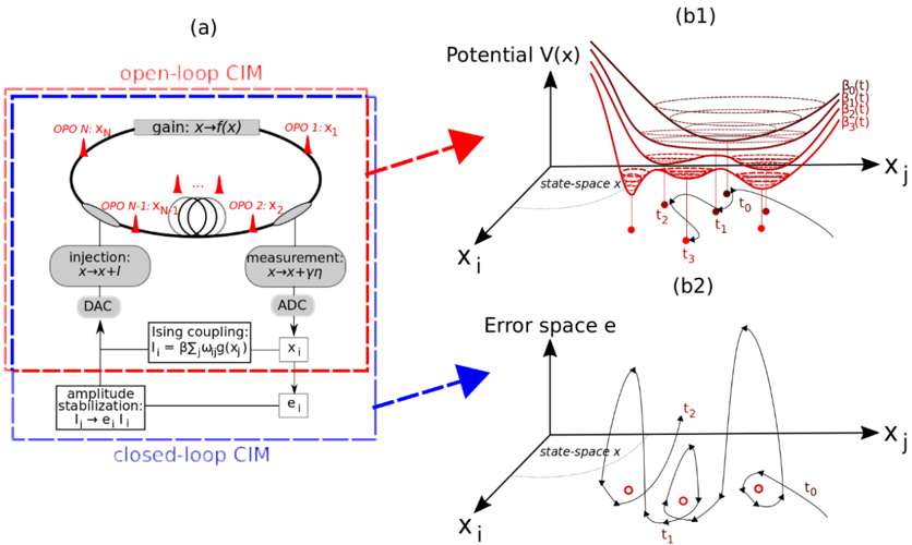
The image presents a diagram illustrating the functional components of an open-loop and closed-loop Computational Ising Machine (CIM), alongside visualizations of the potential energy landscape and error space. The diagram shows the flow of signals and interactions between components, and how feedback is used in the closed-loop system.
### Components/Axes
The diagram is divided into three main sections: (a) Open-loop and Closed-loop CIM, (b1) Potential V(x), and (b2) Error space e.
**Section (a): Open-Loop and Closed-Loop CIM**
* **Open-loop CIM:** Enclosed in a blue dashed rectangle. Contains components labeled:
* OPO 1: X<sub>1</sub>
* OPO 2: X<sub>2</sub>
* OPO N-1: X<sub>N-1</sub>
* OPO N: X<sub>N</sub>
* Injection: x -> x + I (connected to a DAC - Digital to Analog Converter)
* Measurement: x -> x + γn (connected to an ADC - Analog to Digital Converter)
* Ising coupling: I<sub>1</sub> = βΣ<sub>j</sub>ω<sub>ij</sub>g(x<sub>j</sub>)
* Amplitude stabilization: I<sub>1</sub> -> e<sub>1</sub>
* **Closed-loop CIM:** Enclosed in a red dashed rectangle. Contains the same components as the open-loop CIM, with an additional feedback loop from amplitude stabilization (e<sub>1</sub>) to Injection.
* **Arrows:** Red arrows indicate signal flow.
**Section (b1): Potential V(x)**
* **Axes:** X<sub>i</sub> (horizontal) and Potential V(x) (vertical).
* **Visualizations:** Multiple curved lines representing potential energy contours. Red dots are placed along a trajectory labeled t<sub>0</sub>, t<sub>1</sub>, t<sub>2</sub>, t<sub>3</sub>. Several curves are labeled β<sub>0</sub>(t), β<sub>1</sub>(t), β<sub>2</sub>(t), β<sub>3</sub>(t).
* **Text:** "state-space" is written near the origin.
**Section (b2): Error space e**
* **Axes:** X<sub>i</sub> (horizontal) and Error space e (vertical).
* **Visualizations:** Contour lines representing error. A circular trajectory is shown, labeled t<sub>0</sub>, t<sub>1</sub>, t<sub>2</sub>.
* **Text:** "state-space" is written near the origin.
### Detailed Analysis or Content Details
**Section (a): CIM**
The open-loop CIM receives an input 'x' and adds an injection current 'I' via a DAC. The output 'x' is measured with added noise 'γn' via an ADC. The Ising coupling calculates I<sub>1</sub> based on the weighted sum of g(x<sub>j</sub>) with coupling constants ω<sub>ij</sub> and a parameter β. The amplitude stabilization adjusts I<sub>1</sub> to produce e<sub>1</sub>.
The closed-loop CIM adds a feedback loop where e<sub>1</sub> from amplitude stabilization is fed back to the injection stage, creating a closed control system.
**Section (b1): Potential V(x)**
The potential energy landscape shows a multi-dimensional potential with several local minima. The trajectory from t<sub>0</sub> to t<sub>3</sub> indicates a path through the state space, potentially representing the system's evolution towards a lower energy state. The curves β<sub>0</sub>(t) to β<sub>3</sub>(t) likely represent the evolution of a parameter (β) over time.
**Section (b2): Error space e**
The error space shows the error 'e' as a function of X<sub>i</sub>. The circular trajectory from t<sub>0</sub> to t<sub>2</sub> suggests the system oscillates around a stable point, with the error fluctuating within a certain range.
### Key Observations
* The closed-loop CIM incorporates feedback to stabilize the amplitude, suggesting an attempt to improve the system's performance and reduce errors.
* The potential energy landscape (b1) is complex, with multiple local minima, indicating the possibility of getting trapped in suboptimal solutions.
* The error space (b2) shows a relatively stable oscillation, suggesting the feedback mechanism is effective in controlling the error.
* The time labels (t<sub>0</sub>, t<sub>1</sub>, t<sub>2</sub>, t<sub>3</sub>) indicate a temporal evolution of the system's state.
### Interpretation
The diagram illustrates the principles of a Computational Ising Machine and the benefits of using a closed-loop control system. The open-loop CIM is susceptible to noise and instability, while the closed-loop CIM uses feedback to mitigate these issues. The potential energy landscape and error space visualizations provide insights into the system's dynamics and performance. The diagram suggests that the closed-loop CIM is more robust and capable of finding better solutions compared to the open-loop CIM. The trajectory in the potential energy landscape shows the system attempting to minimize its energy, while the trajectory in the error space shows the feedback mechanism keeping the error within acceptable bounds. The diagram is a conceptual representation of the system's functionality and does not provide specific numerical data. It is a high-level overview of the system's architecture and behavior.