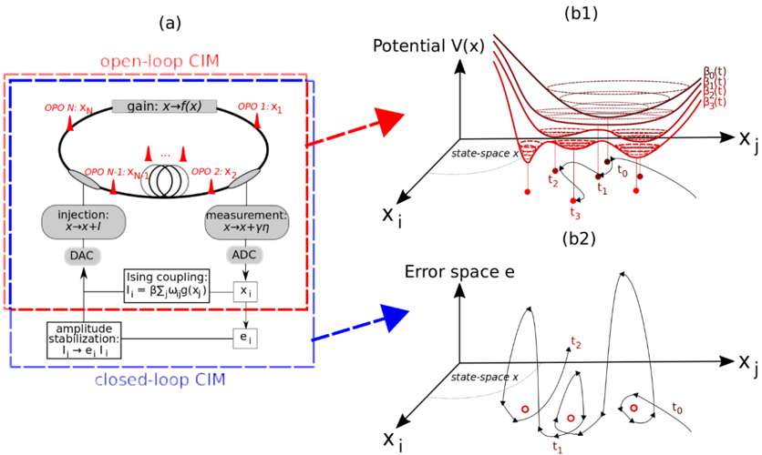
## Diagram: Controlled Ising Machine (CIM) System Architecture and Dynamics
### Overview
The image depicts a technical diagram of a Controlled Ising Machine (CIM) system, illustrating both open-loop and closed-loop configurations, along with graphical representations of potential energy landscapes and error space dynamics. The diagram emphasizes feedback mechanisms, signal processing components, and state-space trajectories.
---
### Components/Axes
#### Diagram (a): CIM System Architecture
- **Open-loop CIM (Red Dashed Box)**:
- **OPOs (Optical Parametric Oscillators)**: Labeled OPO 1 to OPO N, arranged in a feedback loop.
- **Gain**: Labeled "x→f(x)", indicating nonlinear transformation.
- **Injection**: "x→x+l" (input perturbation).
- **Measurement**: "x→x+y" (output sampling).
- **DAC/ADC**: Digital-to-Analog/Analog-to-Digital converters for signal processing.
- **Amplitude Stabilization**: Feedback loop labeled "I_i → e_i I_i" for stabilizing injection signals.
- **Ising Coupling**: Mathematical expression "I_i = βΣ_j ω_j g(x_j)" defining interaction terms.
- **Closed-loop CIM (Blue Dashed Box)**:
- Integrates DAC/ADC and amplitude stabilization into the feedback loop.
#### Graphs (b1) and (b2):
- **Graph (b1): Potential V(x)**:
- **Axes**:
- Vertical: "Potential V(x)" (energy landscape).
- Horizontal: "state-space x" (system state).
- Depth: "X_j" (parameter space).
- **Legend**: Curves labeled β₀(t), β₁(t), β₂(t), β₃(t) represent time-dependent potential wells.
- **Key Features**: Multiple metastable states (wells) and transition paths between them.
- **Graph (b2): Error Space e**:
- **Axes**:
- Vertical: "Error space e" (deviation from desired state).
- Horizontal: "state-space x" (system state).
- Depth: "X_j" (parameter space).
- **Legend**: Trajectories marked with time points t₀, t₁, t₂, t₃.
- **Key Features**: Oscillatory error dynamics and convergence behavior.
---
### Detailed Analysis
#### Diagram (a):
- **Open-loop CIM**:
- OPOs form a closed-loop feedback system with nonlinear gain (x→f(x)).
- Injection (x→x+l) and measurement (x→x+y) processes modulate the system state.
- DAC/ADC enable digital control of analog signals.
- Amplitude stabilization adjusts injection strength (I_i) via error feedback (e_i).
- **Closed-loop CIM**:
- Adds DAC/ADC and amplitude stabilization to refine control, reducing system drift.
#### Graphs (b1) and (b2):
- **Potential V(x) (b1)**:
- Time-dependent potential wells (β₀(t) to β₃(t)) illustrate dynamic energy landscapes.
- Transitions between states (e.g., t₀→t₁→t₂→t₃) suggest metastability and hysteresis.
- **Error Space e (b2)**:
- Trajectories show error oscillations decaying over time (t₀→t₃), indicating stabilization.
- Error magnitude correlates with state-space position (X_j), highlighting parameter sensitivity.
---
### Key Observations
1. **Feedback Mechanisms**:
- Closed-loop CIM introduces DAC/ADC and amplitude stabilization to mitigate errors, contrasting with the open-loop's reliance on passive OPO interactions.
2. **Potential Landscape**:
- Time-varying β(t) curves in (b1) imply adaptive energy minima, critical for solving combinatorial optimization problems.
3. **Error Dynamics**:
- Oscillatory error reduction in (b2) suggests damped feedback control, stabilizing the system near target states.
---
### Interpretation
The diagram illustrates how closed-loop control enhances the CIM's ability to navigate complex, time-dependent energy landscapes. By integrating digital feedback (DAC/ADC) and amplitude stabilization, the system reduces errors and stabilizes trajectories in the error space. The potential V(x) graph highlights the CIM's capacity to explore multiple metastable states, a key feature for solving NP-hard problems like the Ising model. The error dynamics (b2) demonstrate that feedback control suppresses oscillations, ensuring convergence to low-energy states. This architecture bridges analog physical systems (OPOs) with digital control, enabling precise manipulation of quantum-inspired optimization processes.