## Histogram: Bridge Node Persistence Over Time
### Overview
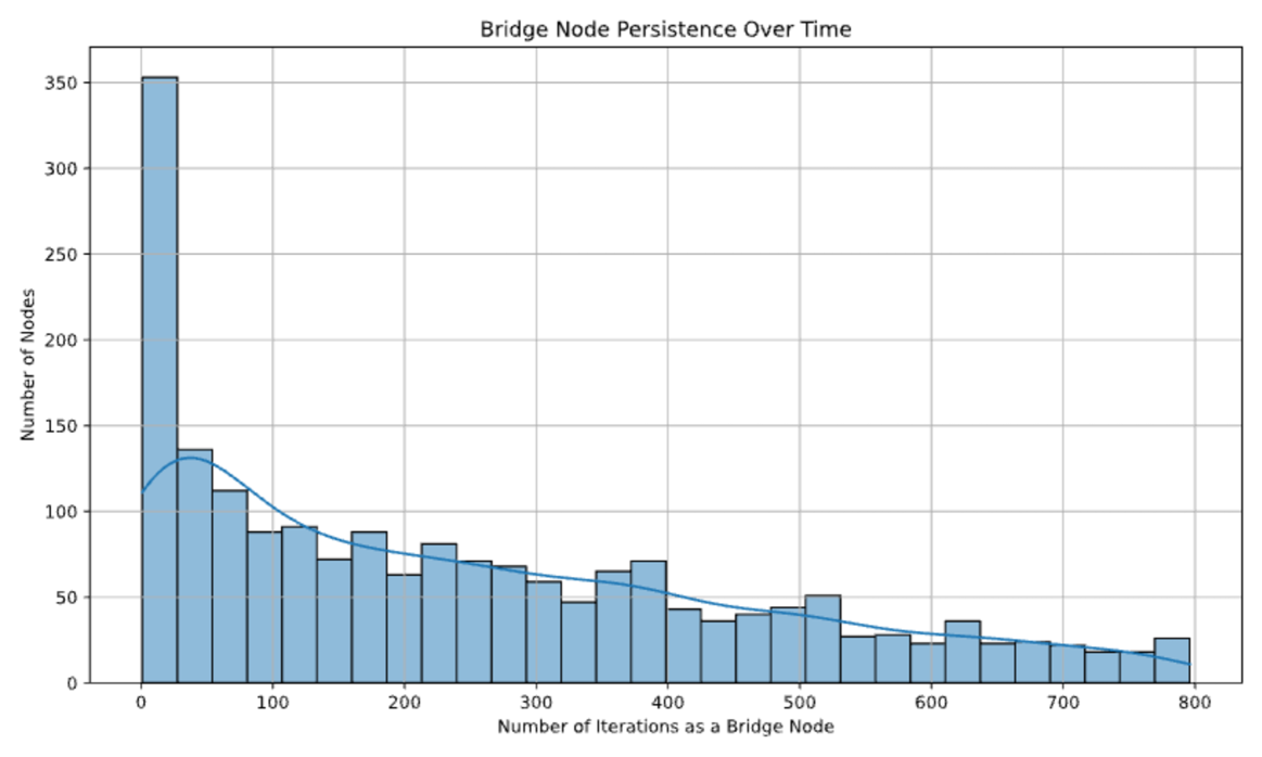
The image displays a histogram representing the distribution of "Bridge Nodes" based on their persistence, measured in "Number of Iterations." The chart features a superimposed blue trend line that illustrates the general decay of node persistence across the dataset. The distribution is heavily right-skewed, indicating that most nodes have a very short lifespan, while a smaller subset persists for a significantly longer duration.
### Components/Axes
* **Title:** "Bridge Node Persistence Over Time" (Centered at the top).
* **X-Axis:** "Number of Iterations as a Bridge Node" (Centered at the bottom).
* Scale: 0 to 800.
* Markers: 0, 100, 200, 300, 400, 500, 600, 700, 800.
* **Y-Axis:** "Number of Nodes" (Centered on the left).
* Scale: 0 to 350.
* Markers: 0, 50, 100, 150, 200, 250, 300, 350.
* **Visual Elements:**
* **Histogram Bars:** Light blue bars with dark blue outlines.
* **Trend Line:** A solid blue curve overlaid on the histogram.
* **Grid:** A light gray grid overlaying the background.
### Detailed Analysis
The histogram is divided into bins of approximately 40 units each.
**Data Distribution (Approximate Values):**
* **The Spike (0-40 iterations):** The first bin is an extreme outlier, reaching approximately 350 nodes.
* **The Decline:** Following the initial spike, the frequency of nodes drops sharply.
* **40-120 iterations:** The count drops from ~135 to ~110.
* **120-400 iterations:** The distribution shows a gradual, fluctuating decline, generally ranging between 90 and 60 nodes per bin.
* **400-800 iterations:** The distribution continues to taper off, with bin heights generally falling between 45 and 20 nodes.
**Trend Line Analysis:**
* **Visual Trend:** The blue trend line slopes upward slightly from x=0 to x=50, then slopes downward continuously toward the right (x=800).
* **Trend Line Values:**
* Starts at x=0, y ≈ 110.
* Peaks at x ≈ 50, y ≈ 130.
* At x=200, y ≈ 80.
* At x=400, y ≈ 60.
* At x=600, y ≈ 30.
* At x=800, y ≈ 15.
### Key Observations
* **Extreme Outlier/Spike:** The first bin (0-40 iterations) contains significantly more nodes (~350) than any other bin. This suggests a high rate of "churn" or transient nodes that disconnect or fail almost immediately after becoming bridge nodes.
* **Trend Line Discrepancy:** There is a notable disconnect between the trend line and the actual data in the first bin. The trend line starts at ~110, while the actual data bar is at ~350. This indicates that the trend line is likely a smoothed statistical model (such as a Kernel Density Estimate) that is heavily influenced by the bulk of the data distribution rather than the extreme initial spike.
* **Long Tail:** The data exhibits a "long tail" distribution, characteristic of systems where a small number of entities (nodes) are highly stable and persist for a long time, while the majority are ephemeral.
### Interpretation
The data demonstrates a classic power-law or exponential decay distribution regarding node stability.
* **System Dynamics:** The system appears to be highly volatile. The vast majority of bridge nodes are short-lived, likely indicating that most nodes are either unstable, malicious, or simply transient participants in the network.
* **Reliability:** The "long tail" extending to 800 iterations suggests that while most nodes are transient, there is a small, reliable core of nodes that maintain persistence over long periods.
* **Modeling Note:** The discrepancy between the trend line and the first histogram bar suggests that the trend line is not a good fit for the "transient" population (the 0-40 iteration group). If the goal of the trend line is to predict node behavior, it significantly underestimates the frequency of short-lived nodes.