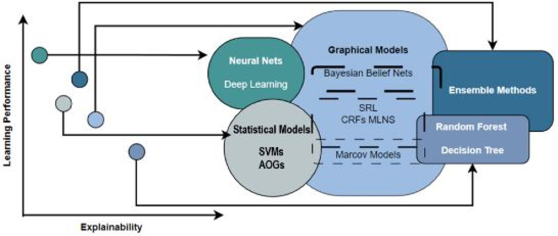
## Diagram: Machine Learning Model Trade-offs (Performance vs. Explainability) ### Overview The diagram illustrates a conceptual map of machine learning models positioned along two axes: **Learning Performance** (vertical) and **Explainability** (horizontal). It categorizes models into four groups—Neural Nets/Deep Learning, Statistical Models (SVMs, AOGs), Graphical Models (Bayesian Belief Nets, SRL, CRFs, MLNS, Markov Models), and Ensemble Methods (Random Forest, Decision Tree)—and shows their relationships via directional arrows. --- ### Components/Axes - **Axes**: - **Vertical (Y-axis)**: Learning Performance (low to high, bottom to top). - **Horizontal (X-axis)**: Explainability (low to high, left to right). - **Key Labels**: - **Neural Nets / Deep Learning** (green circle, top-left quadrant). - **Statistical Models** (light blue circle, bottom-center). - Subcategories: SVMs, AOGs. - **Graphical Models** (dark blue oval, center-right). - Subcategories: Bayesian Belief Nets, SRL, CRFs, MLNS, Markov Models. - **Ensemble Methods** (dark blue rectangle, top-right). - Subcategories: Random Forest, Decision Tree. - **Arrows**: - Indicate relationships (e.g., Neural Nets → Graphical Models → Ensemble Methods). - Dashed lines suggest weaker or indirect connections. --- ### Detailed Analysis 1. **Neural Nets / Deep Learning**: - Positioned at the top-left, indicating **high performance** but **low explainability**. - Connected to Graphical Models via a direct arrow. 2. **Statistical Models (SVMs, AOGs)**: - Located at the bottom-center, reflecting **moderate performance** and **high explainability**. - Dashed lines link to Graphical Models, suggesting limited integration. 3. **Graphical Models**: - Central position (middle-right), balancing **moderate performance** and **moderate explainability**. - Subcategories (e.g., Bayesian Belief Nets, CRFs) are listed within the oval. 4. **Ensemble Methods (Random Forest, Decision Tree)**: - Top-right quadrant, showing **high performance** and **high explainability**. - Connected to Graphical Models via a direct arrow, implying synergy. --- ### Key Observations - **Trade-off**: Models with higher performance (e.g., Neural Nets) sacrifice explainability, while simpler models (e.g., SVMs) prioritize transparency over performance. - **Ensemble Methods** occupy the "sweet spot," balancing both axes. - **Graphical Models** act as a bridge between complex and interpretable models. - **Directional Arrows** suggest a progression from complex (Neural Nets) to hybrid (Graphical Models) to balanced (Ensemble Methods) approaches. --- ### Interpretation The diagram highlights the **performance-explainability trade-off** in machine learning. Neural Nets and Deep Learning dominate in performance but are "black boxes," while Statistical Models (e.g., SVMs) are interpretable but less powerful. Graphical Models (e.g., Bayesian Networks) offer a middle ground, and Ensemble Methods (e.g., Random Forests) combine performance with transparency. The arrows imply that combining techniques (e.g., Neural Nets → Graphical Models → Ensemble Methods) could optimize both axes. Notably, no model achieves peak performance **and** peak explainability simultaneously, underscoring the need for context-specific model selection.