## Chart: Normalization Angle Circular Distributions across Time-steps
### Overview
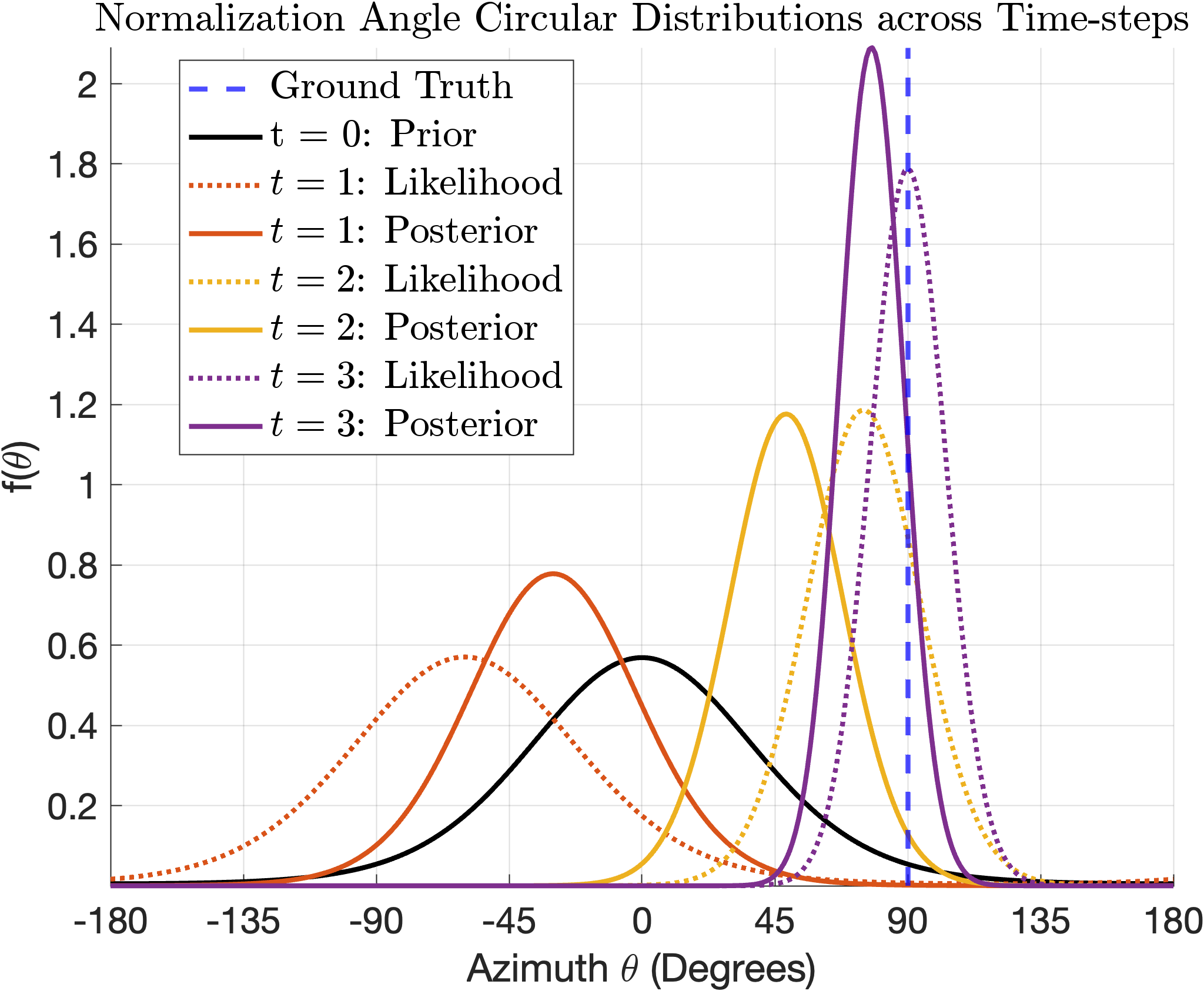
The image presents a line chart illustrating the evolution of probability distributions (circular distributions) of an angle (Azimuth θ) over four time steps (t = 0, 1, 2, 3). The chart compares a "Ground Truth" distribution with prior and posterior distributions calculated at each time step, as well as likelihood distributions at t=1, t=2, and t=3. The y-axis represents the probability density function f(θ).
### Components/Axes
* **Title:** Normalization Angle Circular Distributions across Time-steps
* **X-axis:** Azimuth θ (Degrees), ranging from -180 to 180. Markers are present at -180, -135, -90, -45, 0, 45, 90, 135, and 180.
* **Y-axis:** f(θ) (Probability Density Function), ranging from 0 to 2. Markers are present at 0, 0.2, 0.4, 0.6, 0.8, 1.0, 1.2, 1.4, 1.6, 1.8, and 2.0.
* **Legend:** Located in the top-left corner.
* Ground Truth: Dashed blue line.
* t = 0: Prior: Solid green line.
* t = 1: Likelihood: Dotted orange line.
* t = 1: Posterior: Solid orange line.
* t = 2: Likelihood: Dotted brown line.
* t = 2: Posterior: Solid brown line.
* t = 3: Likelihood: Dotted purple line.
* t = 3: Posterior: Solid purple line.
### Detailed Analysis
The chart displays several curves representing probability distributions.
* **Ground Truth (Dashed Blue):** This distribution is sharply peaked around 90 degrees, with a maximum value of approximately 2.0. It has minimal probability density outside of a narrow range around 90 degrees.
* **t = 0: Prior (Solid Green):** This distribution is relatively flat, with a peak around 0 degrees and a maximum value of approximately 0.5. It has a wider spread than the Ground Truth.
* **t = 1: Likelihood (Dotted Orange):** This distribution is centered around -45 degrees, with a maximum value of approximately 0.6. It is broader than the Ground Truth.
* **t = 1: Posterior (Solid Orange):** This distribution is centered around 45 degrees, with a maximum value of approximately 1.6. It is more concentrated than the Prior and closer to the Ground Truth.
* **t = 2: Likelihood (Dotted Brown):** This distribution is centered around -90 degrees, with a maximum value of approximately 0.4.
* **t = 2: Posterior (Solid Brown):** This distribution is centered around 0 degrees, with a maximum value of approximately 0.8. It is more concentrated than the Likelihood and is shifting towards the Ground Truth.
* **t = 3: Likelihood (Dotted Purple):** This distribution is centered around -45 degrees, with a maximum value of approximately 0.2.
* **t = 3: Posterior (Solid Purple):** This distribution is centered around 90 degrees, with a maximum value of approximately 1.2. It is the closest to the Ground Truth among all posterior distributions.
**Approximate Data Points (extracted visually):**
| Time Step | Distribution | Azimuth (θ) | f(θ) |
|---|---|---|---|
| 0 | Prior | 0 | 0.5 |
| 1 | Likelihood | -45 | 0.6 |
| 1 | Posterior | 45 | 1.6 |
| 2 | Likelihood | -90 | 0.4 |
| 2 | Posterior | 0 | 0.8 |
| 3 | Likelihood | -45 | 0.2 |
| 3 | Posterior | 90 | 1.2 |
| Ground Truth | | 90 | 2.0 |
### Key Observations
* The Prior distribution (t=0) is initially quite diffuse and doesn't resemble the Ground Truth.
* The Likelihood distributions at t=1, t=2, and t=3 are consistently shifted to the left of the Ground Truth.
* The Posterior distributions progressively converge towards the Ground Truth as time steps increase. The posterior at t=3 is the closest approximation.
* The peak of the Posterior distributions shifts from negative angles (t=1) to positive angles (t=3), indicating a learning process.
### Interpretation
This chart demonstrates a Bayesian filtering or state estimation process. The "Ground Truth" represents the actual angle, while the Prior represents an initial belief about the angle. The Likelihood functions represent observations or measurements that provide information about the angle. The Posterior distributions are updated beliefs about the angle, combining the Prior and the Likelihood.
The chart shows how the system learns over time, refining its estimate of the angle based on incoming observations. The convergence of the Posterior distributions towards the Ground Truth indicates that the filtering process is working effectively. The shift in the Likelihood distributions suggests that the measurement process may have a systematic bias or error. The fact that the posterior at t=3 is not *exactly* the ground truth suggests that the system is still imperfect, or that the likelihood function is not perfectly representative of the measurement noise. The chart provides a visual representation of how Bayesian inference can be used to track and estimate a dynamic variable over time.