\n
## Violin Plot: Distribution of Router Stability (Noise γ = 0.01)
### Overview
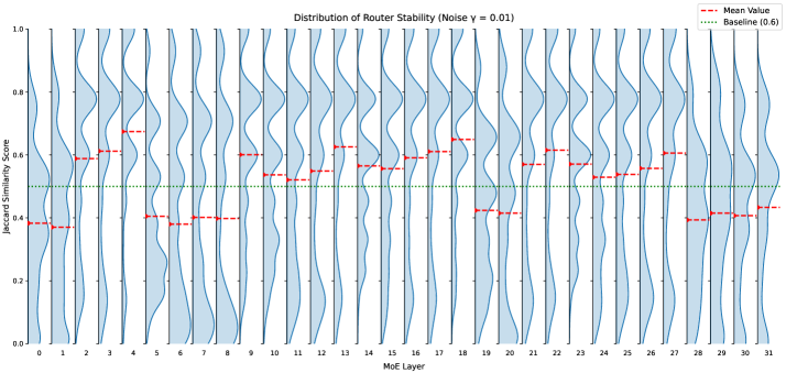
The image is a violin plot visualizing the distribution of router stability scores across 32 distinct layers (0-31) of a Mixture-of-Experts (MoE) model. The stability is measured using the Jaccard Similarity Score under a specific noise condition (γ = 0.01). Each "violin" represents the probability density of the data at different values, with a red dashed line indicating the mean value for that layer. A constant baseline is provided for comparison.
### Components/Axes
* **Chart Title:** "Distribution of Router Stability (Noise γ = 0.01)"
* **X-Axis:**
* **Label:** "MoE Layer"
* **Markers/Ticks:** Integers from 0 to 31, representing individual layers of the model.
* **Y-Axis:**
* **Label:** "Jaccard Similarity Score"
* **Scale:** Linear scale from 0.0 to 1.0, with major ticks at 0.0, 0.2, 0.4, 0.6, 0.8, and 1.0.
* **Legend (Top-Right Corner):**
* **Red dashed line (`---`):** "Mean Value"
* **Green dotted line (`...`):** "Baseline (0.6)"
* **Data Series:** 32 individual violin plots, one per MoE Layer. Each plot is a light blue shaded area representing the data distribution, with a thin black vertical line inside showing the range, and a red horizontal dash marking the mean.
### Detailed Analysis
**Trend Verification:** The mean Jaccard Similarity Score (red dashes) fluctuates across layers without a single monotonic trend. Some layers show higher stability (means above the 0.6 baseline), while others show lower stability (means below the baseline).
**Layer-by-Layer Mean Value Extraction (Approximate):**
* **Layer 0:** Mean ≈ 0.40
* **Layer 1:** Mean ≈ 0.40
* **Layer 2:** Mean ≈ 0.60
* **Layer 3:** Mean ≈ 0.60
* **Layer 4:** Mean ≈ 0.70 (Notably high)
* **Layer 5:** Mean ≈ 0.42
* **Layer 6:** Mean ≈ 0.42
* **Layer 7:** Mean ≈ 0.42
* **Layer 8:** Mean ≈ 0.42
* **Layer 9:** Mean ≈ 0.60
* **Layer 10:** Mean ≈ 0.52
* **Layer 11:** Mean ≈ 0.52
* **Layer 12:** Mean ≈ 0.55
* **Layer 13:** Mean ≈ 0.65
* **Layer 14:** Mean ≈ 0.58
* **Layer 15:** Mean ≈ 0.58
* **Layer 16:** Mean ≈ 0.60
* **Layer 17:** Mean ≈ 0.60
* **Layer 18:** Mean ≈ 0.68 (Notably high)
* **Layer 19:** Mean ≈ 0.42
* **Layer 20:** Mean ≈ 0.42
* **Layer 21:** Mean ≈ 0.58
* **Layer 22:** Mean ≈ 0.58
* **Layer 23:** Mean ≈ 0.52
* **Layer 24:** Mean ≈ 0.52
* **Layer 25:** Mean ≈ 0.52
* **Layer 26:** Mean ≈ 0.60
* **Layer 27:** Mean ≈ 0.60
* **Layer 28:** Mean ≈ 0.40 (Notably low)
* **Layer 29:** Mean ≈ 0.42
* **Layer 30:** Mean ≈ 0.42
* **Layer 31:** Mean ≈ 0.45
**Distribution Shapes:** The violin plots reveal varied distribution characteristics:
* Some layers (e.g., 4, 13, 18) have distributions concentrated at higher Jaccard scores, with means above the baseline.
* Other layers (e.g., 0, 1, 5-8, 19-20, 28-31) have distributions concentrated at lower scores, with means well below the baseline.
* Several layers (e.g., 2, 3, 9, 16-17, 26-27) have distributions centered near the 0.6 baseline.
* The width of the violins indicates the density of data points. Wider sections represent a higher probability of routers in that layer having that specific stability score.
### Key Observations
1. **High-Stability Layers:** Layers 4 and 18 exhibit the highest mean stability (≈0.70 and ≈0.68, respectively), with distributions skewed towards the top of the scale.
2. **Low-Stability Layers:** Layers 0, 1, 28, and 29 show the lowest mean stability (≈0.40-0.42). Layer 28 is particularly notable for its low mean.
3. **Baseline Comparison:** Approximately half of the layers (15 out of 32) have a mean Jaccard score at or below the 0.6 baseline. The other half are above it.
4. **Clustering:** There appears to be clustering of stability profiles. For example, layers 5-8 have nearly identical mean values and similar distribution shapes. Layers 19-20 form another similar pair.
5. **Variability:** The spread (height of the violin) varies significantly. Some layers have a very narrow range of scores (e.g., layer 4), indicating consistent router behavior. Others have a wider spread (e.g., layer 14), indicating more variable router stability under noise.
### Interpretation
This chart provides a diagnostic view of how noise (γ=0.01) affects the routing consistency at each layer of an MoE model. The Jaccard Similarity Score likely measures the overlap between the set of experts selected by a router with and without noise applied.
* **Layer-Specific Robustness:** The data suggests that robustness to noise is not uniform across the model. Early layers (0-1) and very late layers (28-31) appear particularly susceptible to noise, showing low routing stability. Mid-to-late layers (e.g., 4, 13, 18) demonstrate greater robustness.
* **Functional Implications:** Layers with high stability (like 4 and 18) may be performing more critical or robust feature routing, where consistent expert selection is important. Layers with low stability might be more exploratory or sensitive, where noise significantly alters the computation path.
* **Design Insight:** The clustering of similar stability profiles (e.g., layers 5-8) could indicate functional groups within the model architecture. The outlier status of layer 4 (very high stability early on) and layer 28 (very low stability late) warrants further investigation into their specific roles.
* **Baseline Context:** The 0.6 baseline serves as a reference point. The fact that many layers fall below it indicates that a noise level of γ=0.01 is sufficient to disrupt routing consistency in a significant portion of the model. This information is crucial for understanding the model's fault tolerance and for guiding noise-robust training or architecture design.