## Network Diagram: Interconnected Nodes ### Overview The image is a network diagram showing interconnected nodes. The nodes are represented by circles, and the connections between them are represented by curved lines. The color of the nodes and lines varies from light orange to dark red, potentially indicating the strength or frequency of the connection. ### Components/Axes * **Nodes:** Represented by circles of varying sizes and colors. * **Connections:** Represented by curved lines of varying thickness and colors, linking the nodes. * **Color Gradient:** The color of the nodes and lines ranges from light orange to dark red. ### Detailed Analysis * **Node Distribution:** The nodes are clustered in several distinct regions, with some nodes acting as central hubs connecting multiple clusters. * **Connection Density:** The density of connections varies across the diagram, with some regions having a high concentration of lines and others being more sparse. * **Color Variation:** The color of the nodes and lines appears to correlate with the number of connections a node has. Darker red nodes seem to have more connections than lighter orange nodes. * **Hub Nodes:** There are a few prominent nodes that are significantly larger and darker red than the others. These nodes act as central hubs, with many connections radiating from them. One such hub is located in the bottom-left quadrant of the image, and another is in the upper-center. ### Key Observations * The network exhibits a clustered structure, with some nodes acting as central hubs. * The color gradient suggests a correlation between the number of connections and the color intensity of the nodes and lines. * The diagram lacks explicit labels or a legend, making it difficult to determine the exact meaning of the nodes, connections, and color gradient. ### Interpretation The network diagram likely represents a complex system of relationships between different entities. The nodes could represent individuals, organizations, concepts, or any other type of entity, while the connections represent the relationships between them. The color gradient could indicate the strength, frequency, or importance of these relationships. The clustered structure of the network suggests that the entities are grouped into distinct communities or categories. The central hubs represent influential entities that play a key role in connecting these communities. Without additional information, it is difficult to determine the specific meaning of the diagram. However, the visual representation provides valuable insights into the structure and dynamics of the underlying system.

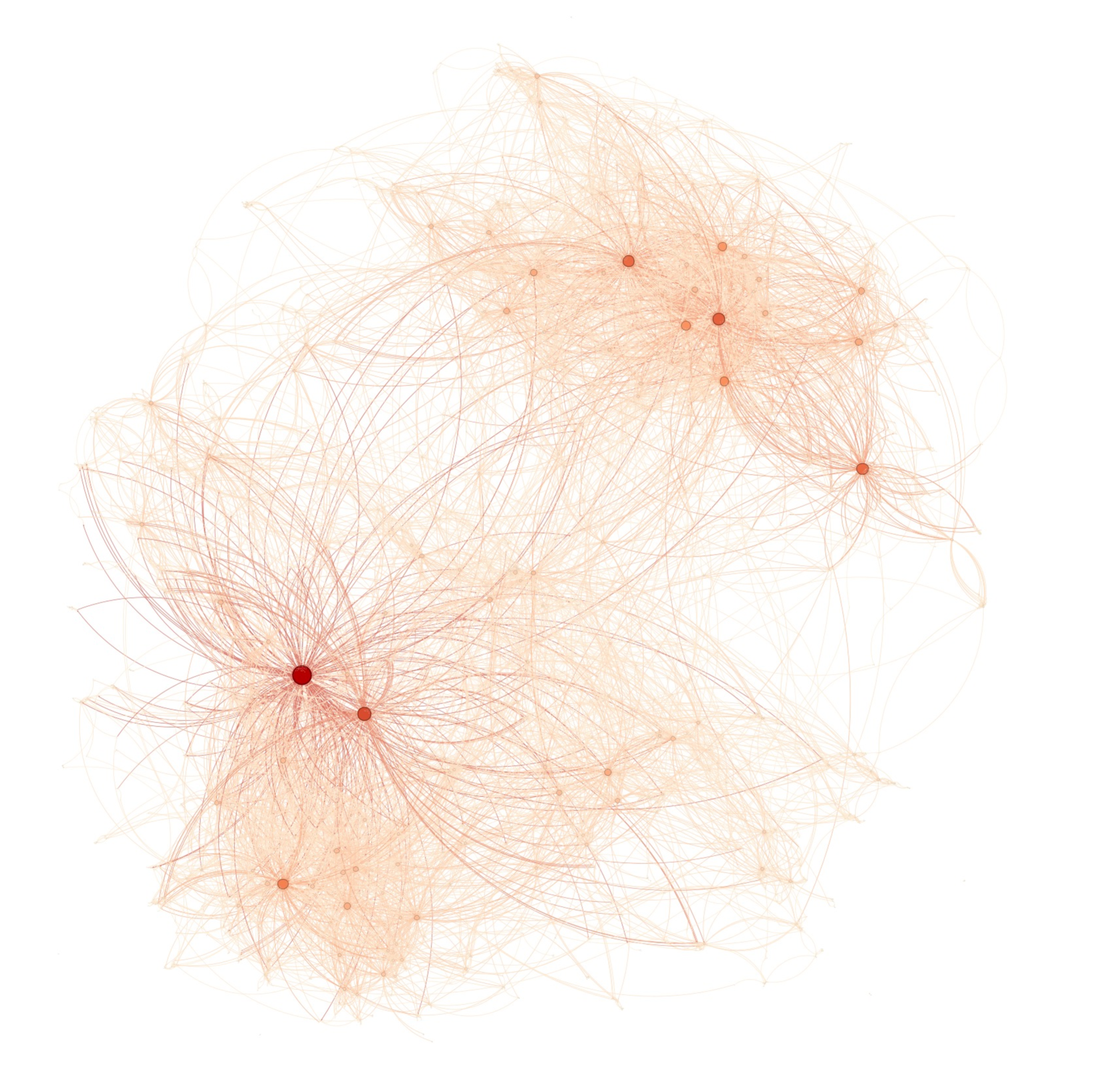
## Network Graph: Bimodal Node-Link Diagram ### Overview This image displays a complex network graph (specifically a node-link diagram) rendered against a solid white background. The visualization maps the relationships and interconnectivity between hundreds to thousands of individual entities. **CRITICAL NOTE:** This image contains absolutely no text, labels, axes, legends, or explicit numerical data. Therefore, specific factual data points (e.g., exact values, categories, or metrics) cannot be extracted. The following analysis is derived entirely from the visual topology, clustering patterns, and the visual encoding (size, color, density) of the network elements. ### Components/Axes In the absence of explicit legends or axes, the data is encoded through the following visual components: * **Nodes (Vertices):** Represented by circular points. * *Size:* Varies significantly. Larger size correlates with a higher number of connections (degree centrality). * *Color:* Ranges from pale, translucent peach/orange (small, peripheral nodes) to deep, opaque crimson red (large, highly connected hub nodes). * **Edges (Links):** Represented by curved lines connecting the nodes. * *Color/Opacity:* Ranges from very faint, translucent peach to darker reddish-brown. Darker lines appear to indicate either higher edge weight (stronger connections) or the visual accumulation of multiple overlapping edges in dense areas. * **Layout:** The spatial distribution appears to be generated by a force-directed layout algorithm. This type of algorithm simulates physical forces, pulling highly connected nodes closer together into clusters while pushing disconnected nodes apart, revealing the underlying structure of the network. ### Detailed Analysis (Spatial Grounding & Component Isolation) To accurately describe the topology, the image can be segmented into distinct spatial regions: **1. Bottom-Left Primary Cluster (The Major Hub)** * *Position:* Centered in the lower-left quadrant of the graph. * *Description:* This is the densest and most visually dominant region of the network. * *Key Features:* It contains the single largest and darkest red node in the entire graph. This node acts as a massive central hub. Immediately to its right (approx. 4 o'clock position relative to the main hub) is a secondary, slightly smaller dark red node. Hundreds of distinct, curved edges radiate outward from these central points in a dense "starburst" or hub-and-spoke pattern, connecting to a vast cloud of smaller, lighter-colored peripheral nodes. **2. Top-Right Secondary Cluster** * *Position:* Located in the upper-right quadrant. * *Description:* A distinct, secondary center of gravity within the network. It is less dense than the bottom-left cluster but highly structured. * *Key Features:* It features one prominent dark red hub node. Unlike the primary cluster, this hub is closely surrounded by a constellation of 4 to 5 medium-sized, moderately red nodes. The connections here form a complex, interconnected web among these medium hubs, rather than a single massive starburst. **3. Far-Right Peripheral Hub** * *Position:* Located on the far right edge, slightly below the horizontal midline. * *Description:* A smaller, isolated sub-cluster. * *Key Features:* It contains one medium-dark red node with a localized, distinct starburst of connections radiating outward, primarily connecting back toward the Top-Right Secondary Cluster. **4. The Interstitial Web (Connecting Tissue)** * *Position:* The space between the major clusters (running diagonally from top-left to bottom-right). * *Description:* This area is characterized by long, sweeping, curved edges that bridge the distinct clusters. * *Key Features:* While the clusters are spatially separated, the dense webbing of faint lines between them indicates that the sub-networks are highly integrated. There are very few isolated nodes; almost everything eventually connects back to the main hubs. ### Key Observations * **Bimodal Distribution:** The network is fundamentally bimodal, dominated by two massive super-clusters (bottom-left and top-right) that dictate the overall shape of the graph. * **Scale-Free Topology:** The visual evidence strongly suggests a "scale-free" network topology. The vast majority of nodes are small and have very few connections, while a tiny minority of nodes (the dark red circles) possess a massive number of connections. * **Curved Edge Bundling:** The edges are drawn as sweeping curves (splines) rather than straight lines. This is a common data visualization technique used to reduce visual clutter in highly dense graphs, allowing the viewer to see the flow of connections without the center becoming a solid, unreadable block of color. ### Interpretation Because we lack the specific data labels, we must interpret the *structural meaning* of this graph. * **System Dynamics:** This topology is typical of systems like social networks (where the red nodes are massive influencers or central figures), biological networks (like protein-protein interactions where central nodes are vital genes), or transportation/routing networks (like major airline hubs). * **Efficiency vs. Vulnerability:** The network is highly efficient for transferring information/resources. Because of the massive central hubs, it likely takes very few "hops" to get from any one node to any other node in the network. However, this structure represents a significant vulnerability. If the single largest node in the bottom-left were removed or failed, that entire half of the network would likely fragment into disconnected pieces. The system relies heavily on a few critical points of failure. * **Community Structure:** The distinct separation between the bottom-left and top-right clusters suggests two distinct "communities" or sub-groups within the broader dataset. While they interact (evidenced by the interstitial web), their internal connections are much stronger than their external connections to each other.

\n ## Network Diagram: Interconnected Nodes ### Overview The image presents a network diagram visualizing relationships between numerous nodes. The diagram consists of a large number of interconnected points (nodes) linked by curved lines (edges). The nodes vary in size, likely representing the importance or degree of connection of each node. The overall structure appears somewhat circular, with denser clusters of nodes in certain areas and sparser connections elsewhere. There are no explicit labels, axes, or legends present in the image. ### Components/Axes There are no axes or explicit labels. The diagram consists solely of nodes and edges. Node size appears to correlate with connectivity. The edges are curved, suggesting a non-Euclidean or force-directed layout. The color scheme is monochromatic, using shades of orange/red. ### Detailed Analysis or Content Details Due to the lack of labels and quantitative data, a precise numerical analysis is impossible. However, we can describe the distribution and characteristics of the network: * **Node Count:** Approximately 200-300 nodes are visible. * **Edge Count:** The number of edges is significantly higher than the node count, indicating a highly connected network. It's difficult to estimate precisely, but likely exceeds 500-800. * **Node Size Distribution:** Node sizes vary considerably. There are a few relatively large nodes (approximately 5-10 with diameters of ~5-10 pixels), many medium-sized nodes (diameter ~2-5 pixels), and a large number of small nodes (diameter < 2 pixels). * **Cluster Identification:** Three main clusters are discernible: * **Bottom-Center Cluster:** This is the most densely connected cluster, with a large central node and numerous connections radiating outwards. * **Top-Left Cluster:** A less dense cluster, but still exhibiting significant internal connectivity. * **Top-Right Cluster:** A smaller, more isolated cluster. * **Edge Density:** Edge density is highest within the bottom-center cluster and lower in the other two clusters. The edges are distributed relatively evenly within each cluster, but there are fewer connections *between* clusters. * **Edge Curvature:** The edges are consistently curved, creating a visually organic and flowing network structure. ### Key Observations * The network exhibits a clear hierarchical structure, with a few central nodes acting as hubs and many peripheral nodes connected to them. * The bottom-center cluster appears to be the most influential or important part of the network. * The top-right cluster is relatively isolated, suggesting it may represent a distinct sub-network or a less integrated component. * The lack of labels makes it impossible to determine the meaning of the nodes and edges. ### Interpretation The diagram likely represents a complex system of relationships, such as a social network, a communication network, or a biological network. The varying node sizes suggest that some entities within the system are more important or have more connections than others. The clusters indicate the presence of distinct groups or communities within the network. The overall structure suggests a degree of centralization, with a few key nodes playing a critical role in connecting the rest of the network. Without additional information, it is difficult to draw more specific conclusions. However, the diagram provides a valuable visual representation of the network's structure and connectivity, which could be used to identify key players, understand the flow of information, or detect potential vulnerabilities. The absence of labels is a significant limitation, but the visual patterns themselves offer insights into the underlying relationships. The diagram is a qualitative visualization, and further analysis would require quantitative data and contextual information.

## Network Graph: Abstract Connectivity Visualization ### Overview The image displays a complex, abstract network graph visualization rendered in a monochromatic orange color palette against a plain white background. It consists of numerous nodes (points) connected by a dense web of curved edges (lines). The visualization appears to be generated by a force-directed layout algorithm, where connected nodes attract each other and all nodes repel each other, resulting in a clustered, organic structure. There is no accompanying text, labels, axes, titles, or legend present in the image. ### Components * **Nodes:** Represented as circular dots. They vary significantly in size and color intensity (saturation/value). * **Size:** Ranges from very small, faint points to large, prominent circles. The largest node is located in the lower-left quadrant. * **Color:** All nodes are shades of orange. Larger nodes are a deeper, more saturated red-orange, while smaller nodes are a pale, light orange. * **Edges:** Represented as thin, curved lines connecting the nodes. They also vary in opacity and thickness. * **Opacity/Thickness:** Lines connected to larger, more central nodes appear darker and slightly thicker. Lines in peripheral or less dense areas are very faint and thin. The curvature suggests an attempt to minimize line crossings in a dense network. * **Spatial Layout:** The graph is not uniformly distributed. It features distinct clusters and several highly connected central hubs. * **Primary Hub:** A very large, dark red-orange node in the lower-left quadrant acts as a major focal point, with a dense starburst of connections radiating from it. * **Secondary Hubs:** Several medium-sized, darker orange nodes are visible, particularly in the upper-right quadrant and near the center, each serving as a local center for their own cluster of connections. * **Periphery:** The outer edges of the graph are populated by many small, faint nodes with fewer connections, creating a diffuse, cloud-like boundary. ### Detailed Analysis * **Node Hierarchy:** The visualization implies a clear hierarchy or importance metric, likely based on **degree centrality** (number of connections). The size and color intensity of a node are directly correlated with its connectivity. * **Largest Node (Lower-Left):** Approximate diameter is 5-7 times that of the smallest nodes. Its deep red-orange color and the sheer density of edges emanating from it mark it as the most significant entity in this network. * **Medium Nodes (e.g., Upper-Right Cluster):** Several nodes are approximately 2-3 times the diameter of the smallest nodes, colored a standard orange. They form the cores of smaller clusters. * **Small Nodes:** The vast majority of nodes are very small and pale, indicating low connectivity. * **Edge Density:** The density of connections is highest around the major hubs, creating visually opaque regions of overlapping lines. The density decreases markedly towards the periphery of the graph. * **Cluster Identification:** At least three major clusters are discernible: 1. A large, dense cluster anchored by the primary hub in the lower-left. 2. A significant cluster in the upper-right quadrant, centered around 2-3 medium hubs. 3. A more diffuse, less tightly knit cluster in the lower-right area. ### Key Observations 1. **Monochromatic Encoding:** All data is encoded using a single hue (orange) with variations in saturation and lightness. This creates a cohesive visual but makes precise differentiation between many nodes challenging without interactive tools. 2. **Absence of Metadata:** The graph is entirely abstract. There are no labels for nodes, no title, no legend explaining what the nodes or edges represent, and no scale. This limits interpretation to structural analysis only. 3. **Force-Directed Layout Characteristics:** The organic, clustered appearance with curved edges is typical of algorithms like Fruchterman-Reingold or Force Atlas, which prioritize showing community structure and relative importance. 4. **Visual Weight Imbalance:** The composition is heavily weighted towards the lower-left due to the primary hub, creating a strong visual anchor point. ### Interpretation This image is a pure visualization of **network topology and relative node importance**. It demonstrates the following structural principles: * **Scale-Free Network Properties:** The presence of a few highly connected hubs (the large nodes) amidst many poorly connected nodes is characteristic of scale-free networks, common in social networks, biological pathways, and the internet. * **Community Structure:** The clear clustering indicates the network contains communities or modules—groups of nodes more densely connected to each other than to the rest of the network. * **Centrality Visualization:** The design effectively uses pre-attentive visual attributes (size, color intensity) to immediately draw the viewer's eye to the most central nodes, providing an instant understanding of the network's backbone. **Limitations & Missing Information:** The complete lack of semantic labels is the critical limitation. We cannot determine if this represents a social network, a citation network, a neural network, a protein interaction map, or any other type of relational data. The visualization shows *that* structure exists and *what* its relative properties are, but not *what it is*. To derive factual meaning, this graph would need to be paired with a data table mapping node IDs to labels and a description of the edge relationships.

## Network Diagram: Abstract Connectivity Web ### Overview The image depicts a complex network of interconnected nodes and pathways. Nodes are represented as red circular points, while connections are thin, light-colored lines forming a dense, web-like structure. The layout is organic, with no rigid geometric constraints, suggesting a dynamic or emergent system. ### Components/Axes - **Nodes**: Red circular points scattered throughout the diagram. - **Connections**: Thin, light-colored lines linking nodes. - **No explicit labels, legends, or axis markers** are present. - **No numerical scales, categories, or textual annotations** are visible. ### Detailed Analysis - **Node Distribution**: - Nodes are unevenly distributed, with clusters in the upper-right and lower-left regions. - A central node (bright red) acts as a focal point, radiating connections to surrounding nodes. - Smaller nodes (darker red) are dispersed in peripheral areas, with fewer connections. - **Connection Density**: - High-density regions (e.g., upper-right cluster) show overlapping lines, creating a "hairball" effect. - Lower-density areas (e.g., lower-left) have sparser, more isolated connections. - **Color Gradient**: - Nodes transition from bright red (central) to darker red (peripheral), possibly indicating hierarchy or activity level. - Lines are uniformly light beige, with no variation in thickness or color. ### Key Observations 1. **Central Hub**: The bright red node in the lower-left quadrant dominates the network, suggesting a primary node or hub. 2. **Clustered Regions**: The upper-right cluster exhibits the highest connection density, implying a sub-network or community. 3. **Peripheral Isolation**: Nodes in the lower-right and upper-left corners have minimal connections, indicating potential outliers or isolated components. 4. **No Textual Elements**: No labels, legends, or axis titles are present, limiting direct interpretation of node identities or relationships. ### Interpretation This diagram likely represents a network analysis of a system with hierarchical or community-based structures. The central hub and clustered regions suggest key nodes or groups with high interconnectivity, while peripheral nodes may represent less critical or isolated elements. The absence of labels or legends prevents definitive identification of nodes or their roles. The organic layout implies a focus on relational dynamics rather than quantitative metrics. **Note**: The image contains no textual information, numerical data, or explicit labels. All interpretations are based on visual patterns and spatial relationships.