## Charts: MSC vs. kHz for Various Algorithms
### Overview
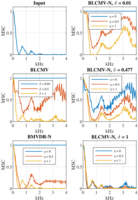
The image presents six charts displaying Modified Spectral Correlation (MSC) values against frequency in kHz. Each chart represents a different algorithm or parameter setting, with lines representing different values of η (eta) or δ (delta). The top-left chart shows the input signal's MSC. The remaining charts show the MSC for different algorithms (BLCMV-N, BLCMV, BMVDR-N, BLCMV-N) and parameter settings.
### Components/Axes
All charts share the following components:
* **X-axis:** Frequency in kHz, ranging from 0 to 4 kHz. The axis is labeled "kHz".
* **Y-axis:** Modified Spectral Correlation (MSC), ranging from 0 to 1. The axis is labeled "MSC".
* **Legends:** Each chart has a legend indicating the different lines and their corresponding η or δ values.
* **Titles:** Each chart has a title indicating the algorithm and parameter settings.
Specific chart details:
1. **Top-Left: Input** - Displays the MSC of the input signal.
2. **Top-Right: BLCMV-N, δ = 0.01** - Shows MSC vs. kHz for BLCMV-N with δ fixed at 0.01 and varying η (0, 0.5, 1).
3. **Middle-Left: BLCMV, δ = 0.01 & δ = 0.5** - Shows MSC vs. kHz for BLCMV with δ values of 0.01 and 0.5, and a single η value.
4. **Middle-Right: BLCMV-N, δ = 0.477** - Shows MSC vs. kHz for BLCMV-N with δ fixed at 0.477 and varying η (0, 0.5, 1).
5. **Bottom-Left: BMVDR-N** - Shows MSC vs. kHz for BMVDR-N with varying η (0, 0.5, 1).
6. **Bottom-Right: BLCMV-N, δ = 1** - Shows MSC vs. kHz for BLCMV-N with δ fixed at 1 and varying η (0, 0.5, 1).
### Detailed Analysis or Content Details
**1. Input:**
* The line (blue) starts at approximately 0.8 at 0 kHz, rapidly decreases to approximately 0.1 at 1 kHz, and remains relatively flat around 0.1 until 4 kHz.
**2. BLCMV-N, δ = 0.01:**
* η = 0 (red): Starts at approximately 0.8, drops sharply to around 0.5 at 0.5 kHz, then fluctuates between 0.5 and 0.7, peaking around 3 kHz at approximately 0.75.
* η = 0.5 (orange): Starts at approximately 0.8, drops to around 0.5 at 0.5 kHz, and then gradually increases to approximately 0.65 at 4 kHz.
* η = 1 (blue): Starts at approximately 0.8, drops to around 0.5 at 0.5 kHz, and then fluctuates between 0.5 and 0.6, peaking around 3 kHz at approximately 0.6.
**3. BLCMV, δ = 0.01 & δ = 0.5:**
* δ = 0.01 (red): Starts at approximately 0.8, drops to around 0.4 at 0.5 kHz, and then fluctuates between 0.4 and 0.6, peaking around 3 kHz at approximately 0.6.
* δ = 0.5 (orange): Starts at approximately 0.8, drops to around 0.3 at 0.5 kHz, and then fluctuates between 0.3 and 0.5, peaking around 3 kHz at approximately 0.5.
**4. BLCMV-N, δ = 0.477:**
* η = 0 (red): Starts at approximately 0.8, drops to around 0.5 at 0.5 kHz, and then fluctuates between 0.5 and 0.7, peaking around 3 kHz at approximately 0.7.
* η = 0.5 (orange): Starts at approximately 0.8, drops to around 0.5 at 0.5 kHz, and then gradually increases to approximately 0.65 at 4 kHz.
* η = 1 (blue): Starts at approximately 0.8, drops to around 0.5 at 0.5 kHz, and then fluctuates between 0.5 and 0.6, peaking around 3 kHz at approximately 0.6.
**5. BMVDR-N:**
* η = 0 (red): Starts at approximately 0.8, drops to around 0.4 at 0.5 kHz, and then remains relatively flat around 0.4 until 4 kHz.
* η = 0.5 (orange): Starts at approximately 0.8, drops to around 0.4 at 0.5 kHz, and then remains relatively flat around 0.4 until 4 kHz.
* η = 1 (blue): Starts at approximately 0.8, drops to around 0.4 at 0.5 kHz, and then remains relatively flat around 0.4 until 4 kHz.
**6. BLCMV-N, δ = 1:**
* η = 0 (red): Starts at approximately 0.8, drops sharply to around 0.5 at 0.5 kHz, and then fluctuates between 0.5 and 0.7, peaking around 3 kHz at approximately 0.7.
* η = 0.5 (orange): Starts at approximately 0.8, drops to around 0.5 at 0.5 kHz, and then gradually increases to approximately 0.65 at 4 kHz.
* η = 1 (blue): Starts at approximately 0.8, drops to around 0.5 at 0.5 kHz, and then fluctuates between 0.5 and 0.6, peaking around 3 kHz at approximately 0.6.
### Key Observations
* The input signal has a significantly higher MSC value at low frequencies compared to the other algorithms.
* All algorithms show a general decrease in MSC at lower frequencies (below 1 kHz).
* The parameter η seems to have a more pronounced effect on the MSC values for BLCMV-N and BLCMV algorithms than for BMVDR-N.
* The δ parameter significantly impacts the MSC values for BLCMV and BLCMV-N algorithms.
* BMVDR-N shows minimal variation in MSC across different η values.
### Interpretation
The charts demonstrate the performance of different algorithms in estimating the Modified Spectral Correlation (MSC) of a signal across various frequencies. The input signal's MSC profile serves as a baseline for comparison. The variations in MSC values observed for different algorithms and parameter settings (η and δ) suggest that these parameters play a crucial role in shaping the MSC estimation.
The fact that BMVDR-N exhibits minimal sensitivity to η indicates that its performance is relatively stable regardless of this parameter. Conversely, the noticeable variations in MSC values for BLCMV-N and BLCMV algorithms with different η values suggest that this parameter can be tuned to optimize performance.
The impact of the δ parameter on BLCMV and BLCMV-N algorithms highlights its importance in controlling the algorithm's behavior. The different δ values lead to distinct MSC profiles, indicating that selecting an appropriate δ value is critical for achieving desired performance.
The overall trend of decreasing MSC at lower frequencies across all algorithms suggests that these algorithms may be less effective at capturing signal correlations at lower frequencies. The fluctuations in MSC values at higher frequencies may indicate the presence of noise or other artifacts in the signal.