## Line Graphs: Comparative Analysis of MSC Across Parameters
### Overview
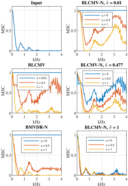
The image contains six line graphs arranged in two columns and three rows, comparing the Mean Squared Coefficient (MSC) across frequency (kHz) for different parameter configurations. Each graph includes legends with η values (0, 0.5, 1) and varying δ parameters (0.01, 0.477, 1). The graphs are labeled as follows:
- **Top Row**: "Input" (left), "BLCMV-N, δ = 0.01" (right)
- **Middle Row**: "BLCMV" (left), "BLCMV-N, δ = 0.477" (right)
- **Bottom Row**: "BMVDR-N" (left), "BLCMV-N, δ = 1" (right)
### Components/Axes
- **X-Axis**: Labeled "kHz" with a range of 0–4 kHz.
- **Y-Axis**: Labeled "MSC" with a range of 0–1.
- **Legends**: Positioned in the top-right corner of each graph, showing η values (0 = blue, 0.5 = red, 1 = yellow). All graphs include these three η values, though some graphs (e.g., "Input") only display one line (η = 0).
- **Graph Titles**: Located at the top of each graph, specifying the model and δ parameter (e.g., "BLCMV-N, δ = 0.01").
### Detailed Analysis
#### Input Graph (Top-Left)
- **Lines**: Single blue line (η = 0).
- **Trend**: Sharp drop from MSC = 1 to ~0.1 between 0–1 kHz, then stabilizes near 0.
- **Key Points**:
- At 0 kHz: MSC ≈ 1.0
- At 1 kHz: MSC ≈ 0.1
- At 4 kHz: MSC ≈ 0.0
#### BLCMV-N, δ = 0.01 (Top-Right)
- **Lines**:
- Blue (η = 0): Sharp drop to ~0.1 by 1 kHz, then stabilizes.
- Red (η = 0.5): Peaks at ~0.8 MSC around 1.5 kHz, then declines.
- Yellow (η = 1): Peaks at ~0.6 MSC around 2.5 kHz, then declines.
- **Key Points**:
- η = 0.5 peak: 1.5 kHz, MSC ≈ 0.8
- η = 1 peak: 2.5 kHz, MSC ≈ 0.6
#### BLCMV (Middle-Left)
- **Lines**:
- Blue (η = 0): Sharp drop to ~0.1 by 1 kHz, then stabilizes.
- Red (η = 0.5): Oscillates between 0.3–0.7 MSC up to 3 kHz.
- Yellow (η = 1): Oscillates between 0.1–0.5 MSC up to 4 kHz.
- **Key Points**:
- η = 0.5: Peaks at ~0.7 MSC around 2 kHz.
- η = 1: Peaks at ~0.5 MSC around 3 kHz.
#### BLCMV-N, δ = 0.477 (Middle-Right)
- **Lines**:
- Blue (η = 0): Sharp drop to ~0.1 by 1 kHz, then stabilizes.
- Red (η = 0.5): Oscillates between 0.4–0.8 MSC up to 3 kHz.
- Yellow (η = 1): Oscillates between 0.2–0.6 MSC up to 4 kHz.
- **Key Points**:
- η = 0.5: Peaks at ~0.8 MSC around 2.5 kHz.
- η = 1: Peaks at ~0.6 MSC around 3.5 kHz.
#### BMVDR-N (Bottom-Left)
- **Lines**:
- Blue (η = 0): Sharp drop to ~0.1 by 1 kHz, then stabilizes.
- Red (η = 0.5): Peaks at ~0.7 MSC around 1.5 kHz, then declines.
- Yellow (η = 1): Peaks at ~0.5 MSC around 2.5 kHz, then declines.
- **Key Points**:
- η = 0.5 peak: 1.5 kHz, MSC ≈ 0.7
- η = 1 peak: 2.5 kHz, MSC ≈ 0.5
#### BLCMV-N, δ = 1 (Bottom-Right)
- **Lines**:
- Blue (η = 0): Sharp drop to ~0.1 by 1 kHz, then stabilizes.
- Red (η = 0.5): Sharp drop to ~0.3 by 1.5 kHz, then oscillates between 0.2–0.4.
- Yellow (η = 1): Sharp drop to ~0.2 by 1.5 kHz, then oscillates between 0.1–0.3.
- **Key Points**:
- η = 0.5: Peaks at ~0.3 MSC around 2 kHz.
- η = 1: Peaks at ~0.3 MSC around 3 kHz.
### Key Observations
1. **Input Baseline**: The "Input" graph shows a universal sharp drop in MSC, serving as a reference for unmodified signals.
2. **δ Parameter Impact**: Higher δ values (e.g., δ = 1) result in sharper MSC drops and reduced oscillations compared to lower δ values (e.g., δ = 0.01).
3. **η Parameter Impact**:
- η = 0.5 and η = 1 introduce frequency-dependent oscillations, with peaks shifting to higher frequencies as η increases.
- η = 0.5 consistently shows higher MSC peaks than η = 1 across most graphs.
4. **Model-Specific Behavior**:
- **BLCMV-N**: δ modulates the sharpness of the MSC drop and the amplitude of oscillations.
- **BLCMV**: η introduces sustained oscillations without δ influence.
- **BMVDR-N**: η = 0.5 and η = 1 exhibit similar peak frequencies but lower amplitudes compared to BLCMV-N variants.
### Interpretation
The data demonstrates that:
- **δ** acts as a threshold parameter, controlling the initial MSC drop and the persistence of oscillations. Higher δ values suppress oscillations more aggressively.
- **η** modulates the frequency response, with higher η values shifting peak MSC to higher frequencies and reducing peak amplitudes.
- The "Input" graph establishes a baseline MSC profile, while parameterized models (BLCMV-N, BLCMV, BMVDR-N) show how η and δ jointly shape the MSC across frequencies. This suggests δ fine-tunes the system's sensitivity, while η adjusts the frequency-dependent behavior.
- Outliers (e.g., sharp peaks in BLCMV-N, δ = 0.01) indicate resonant frequencies where η amplifies the MSC, potentially highlighting critical operational thresholds.