## Diagram: Machine Learning Loss Function Flowchart
### Overview
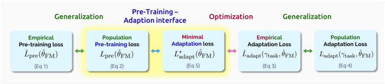
The image displays a horizontal flowchart illustrating the relationship between different loss functions in a machine learning model's training and adaptation process. The diagram progresses from left to right, showing a sequence of five rectangular boxes connected by colored, double-headed arrows. The flow emphasizes transitions between empirical and population losses, and between pre-training and task-specific adaptation phases.
### Components/Axes
The diagram consists of five main components (boxes) arranged linearly:
1. **Box 1 (Far Left):**
* **Label:** `Empirical Pre-training loss`
* **Equation:** `L_pre(θ_FM)`
* **Reference:** `(Eq 1)`
* **Position:** Leftmost box.
2. **Box 2 (Center-Left):**
* **Label:** `Population Pre-training loss`
* **Equation:** `L_pre(θ_FM)`
* **Reference:** `(Eq 2)`
* **Position:** Second from left. This box has a distinct yellow highlight/background.
3. **Box 3 (Center):**
* **Label:** `Minimal Adaptation loss` (The word "Minimal" is in red text).
* **Equation:** `L*_adapt(θ_FM)`
* **Reference:** `(Eq 5)`
* **Position:** Central box.
4. **Box 4 (Center-Right):**
* **Label:** `Empirical Adaptation Loss`
* **Equation:** `L_adapt(T_task, θ_FM)`
* **Reference:** `(Eq 3)`
* **Position:** Fourth from left.
5. **Box 5 (Far Right):**
* **Label:** `Population Adaptation Loss`
* **Equation:** `L_adapt(T_task, θ_FM)`
* **Reference:** `(Eq 4)`
* **Position:** Rightmost box.
**Connecting Arrows:**
* **Between Box 1 & 2:** A green, double-headed arrow.
* **Between Box 2 & 3:** A blue, double-headed arrow.
* **Between Box 3 & 4:** A red, double-headed arrow.
* **Between Box 4 & 5:** A green, double-headed arrow.
**Overarching Labels (Positioned above the boxes):**
* Above Box 1: `Generalization` (in green text).
* Above the space between Box 2 & 3: `Pre-Training - Adaption interface` (in blue text).
* Above Box 3 & 4: `Optimization` (in red text).
* Above Box 5: `Generalization` (in green text).
### Detailed Analysis
The diagram maps a conceptual pathway for model training:
1. **Pre-Training Phase (Left Side):** Starts with the `Empirical Pre-training loss` (Eq 1), which is the loss calculated on the actual pre-training dataset. This is connected to the `Population Pre-training loss` (Eq 2), representing the theoretical loss over the entire data distribution. The green arrow and the "Generalization" label above suggest this transition is about the model's ability to generalize from the training sample to the broader population.
2. **Interface & Adaptation (Center):** The `Population Pre-training loss` connects via a blue arrow to the `Minimal Adaptation loss` (Eq 5). This central box, highlighted in yellow, represents the optimal point of adaptation. The blue label "Pre-Training - Adaption interface" indicates this is the bridge between the general pre-trained model and task-specific tuning.
3. **Adaptation Phase (Right Side):** The `Minimal Adaptation loss` connects via a red arrow to the `Empirical Adaptation Loss` (Eq 3), which is the loss on the specific task's training data (`T_task`). This is labeled as "Optimization," indicating the process of fitting the model to the new task. Finally, this connects via another green arrow to the `Population Adaptation Loss` (Eq 4), the generalization of the adapted model to the full task distribution, again under a "Generalization" label.
### Key Observations
* **Symmetry in Generalization:** The process begins and ends with a "Generalization" step (green arrows), moving from an empirical loss to a population loss in both the pre-training and adaptation phases.
* **Central Pivot Point:** The `Minimal Adaptation loss` (Eq 5) is the central, highlighted node. It acts as the pivot between the pre-training world (left) and the task-specific adaptation world (right).
* **Color-Coded Semantics:** Colors are used consistently to denote concepts: Green for generalization, Blue for the pre-training/adaptation interface, and Red for optimization/minimal loss.
* **Equation Reference:** Each loss function is tied to a specific equation number (Eq 1-5), indicating this diagram is likely from a technical paper or report where these equations are formally defined.
* **Notation Consistency:** The model parameters are consistently denoted as `θ_FM` across all loss functions, suggesting a fixed model backbone being adapted.
### Interpretation
This diagram provides a conceptual framework for understanding the theoretical underpinnings of transfer learning or foundation model adaptation. It visually argues that successful adaptation involves more than just minimizing a task-specific empirical loss (Eq 3). The key is finding the `Minimal Adaptation loss` (Eq 5), which serves as an optimal interface point derived from the pre-trained model's population loss (Eq 2). This point then allows for effective generalization to the new task's population (Eq 4).
The flow suggests a Peircean investigative logic: moving from specific observations (Empirical Pre-training loss) to a general law or hypothesis (Population Pre-training loss), then using that to find an optimal rule for a new situation (Minimal Adaptation loss), which is tested on new specific data (Empirical Adaptation Loss) to confirm its general applicability (Population Adaptation Loss). The diagram emphasizes that robust adaptation is a structured process of generalization, interface, optimization, and re-generalization, not merely a single step of fine-tuning.