## Flowchart: Pre-Training – Adaptation Interface Workflow
### Overview
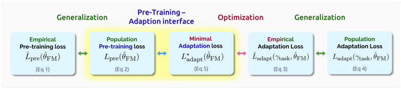
The image depicts a five-stage workflow for model adaptation, emphasizing generalization, pre-training, optimization, and adaptation. The process begins and ends with "Generalization," with intermediate stages involving pre-training, adaptation interface, and optimization. Color-coded boxes and arrows indicate distinct phases and relationships.
### Components/Axes
- **Title**: "Pre-Training – Adaptation interface" (centered, blue text).
- **Boxes**:
1. **Empirical Pre-training Loss** (light blue, green text):
- Label: `L̂_pre(θ̂_FM)` (Equation 1).
2. **Population Pre-training Loss** (light blue, green text):
- Label: `L_pre(θ̂_FM)` (Equation 2).
3. **Minimal Adaptation Loss** (light blue, red text):
- Label: `L*_adapt(θ̂_FM)` (Equation 5).
4. **Empirical Adaptation Loss** (light blue, red text):
- Label: `L̂_adapt(γ_task, θ̂_FM)` (Equation 3).
5. **Population Adaptation Loss** (light blue, green text):
- Label: `L_adapt(γ_task, θ̂_FM)` (Equation 4).
- **Arrows**:
- Green arrows: Connect "Empirical Pre-training Loss" → "Population Pre-training Loss" → "Empirical Adaptation Loss" → "Population Adaptation Loss."
- Blue arrows: Connect "Population Pre-training Loss" → "Minimal Adaptation Loss."
- Red arrow: Connect "Minimal Adaptation Loss" → "Empirical Adaptation Loss."
- **Legend**: Implicit color coding (green = generalization, blue = pre-training/adaptation interface, red = optimization).
### Detailed Analysis
1. **Stage 1 (Generalization)**:
- **Empirical Pre-training Loss** (`L̂_pre(θ̂_FM)`) and **Population Pre-training Loss** (`L_pre(θ̂_FM)`) are grouped under "Generalization" (green).
- Both use the same parameter `θ̂_FM` but differ in empirical vs. population loss formulations.
2. **Stage 2 (Pre-Training – Adaptation Interface)**:
- **Population Pre-training Loss** (`L_pre(θ̂_FM)`) transitions via a blue arrow to **Minimal Adaptation Loss** (`L*_adapt(θ̂_FM)`), suggesting optimization toward minimizing adaptation error.
3. **Stage 3 (Optimization)**:
- **Minimal Adaptation Loss** (`L*_adapt(θ̂_FM)`) is connected to **Empirical Adaptation Loss** (`L̂_adapt(γ_task, θ̂_FM)`) via a red arrow, indicating a refinement step.
4. **Stage 4 (Generalization)**:
- **Empirical Adaptation Loss** and **Population Adaptation Loss** (`L_adapt(γ_task, θ̂_FM)`) are grouped under "Generalization" (green), emphasizing task-specific adaptation.
### Key Observations
- The workflow cycles from generalization to optimization and back, implying iterative refinement.
- **Empirical** and **Population** losses are differentiated by color (green vs. red) and equation structure (e.g., `L̂` vs. `L`).
- The **Minimal Adaptation Loss** (`L*_adapt`) acts as a bridge between pre-training and adaptation, highlighting optimization as a critical step.
### Interpretation
The diagram illustrates a model adaptation pipeline where:
1. **Pre-training** (generalization phase) establishes a foundational model (`θ̂_FM`).
2. **Optimization** (via minimal adaptation loss) refines the model to reduce task-specific errors.
3. **Adaptation** (empirical/population) tailors the model to specific tasks (`γ_task`), balancing generalization and specialization.
- **Color coding** suggests a hierarchy: green (broad generalization), blue (intermediate adaptation), red (fine-grained optimization).
- The use of `θ̂_FM` across stages implies parameter updates propagate through the workflow, with `γ_task` representing task-specific constraints.
This structure emphasizes the interplay between pre-training for generalization and adaptation for task-specific performance, with optimization ensuring efficient convergence.