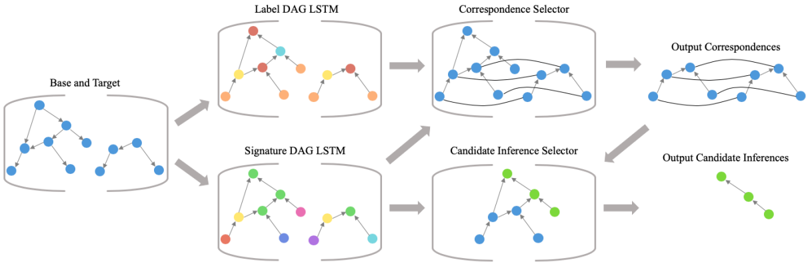
\n ## Diagram: Dual-Path DAG LSTM Architecture for Correspondence and Inference Generation ### Overview The image is a technical system architecture diagram illustrating a two-pathway machine learning pipeline. The process begins with a combined input and splits into parallel processing streams that use Directed Acyclic Graph (DAG) Long Short-Term Memory (LSTM) networks. These streams converge into selector modules, ultimately producing two distinct types of output: "Output Correspondences" and "Output Candidate Inferences." The flow is strictly left-to-right, indicated by gray arrows. ### Components/Axes The diagram is composed of six primary labeled components, connected by directional arrows. There are no traditional chart axes, legends, or numerical data points. The components are: 1. **Base and Target** (Far Left): The initial input module. 2. **Label DAG LSTM** (Top Center-Left): The first parallel processing unit. 3. **Signature DAG LSTM** (Bottom Center-Left): The second parallel processing unit. 4. **Correspondence Selector** (Top Center-Right): The module that processes the output from the Label DAG LSTM. 5. **Candidate Inference Selector** (Bottom Center-Right): The module that processes outputs from both the Signature DAG LSTM and the Correspondence Selector. 6. **Output Correspondences** (Top Right): The final output of the top pathway. 7. **Output Candidate Inferences** (Bottom Right): The final output of the bottom pathway. ### Detailed Analysis The process flow and component relationships are as follows: 1. **Input Stage**: The process starts at the **"Base and Target"** component. This module contains a visual representation of two interconnected graph structures (blue nodes and edges), suggesting the input data consists of two related graph-based entities. 2. **Parallel Processing Stage**: The input data splits into two separate processing paths: * **Top Path**: Data flows into the **"Label DAG LSTM"**. This component contains two graph structures. The left graph has nodes colored red, yellow, and blue. The right graph has nodes colored red, orange, and blue. The title suggests this network processes label information within a DAG structure. * **Bottom Path**: Data flows into the **"Signature DAG LSTM"**. This component also contains two graph structures. The left graph has nodes colored green, yellow, and red. The right graph has nodes colored green, pink, blue, and cyan. The title suggests this network processes signature or structural feature information. 3. **Selection and Integration Stage**: The outputs from the parallel LSTMs are fed into selector modules: * The output of the **Label DAG LSTM** goes to the **"Correspondence Selector"**. This module shows a complex, merged graph structure with blue nodes, indicating it is synthesizing information to find correspondences. * The output of the **Signature DAG LSTM** goes to the **"Candidate Inference Selector"**. This module also shows a merged graph structure with blue and green nodes. Crucially, it also receives a direct input arrow from the **"Correspondence Selector"**, indicating a dependency where inference selection uses the results of correspondence selection. 4. **Output Stage**: The final modules produce the system's results: * The **"Correspondence Selector"** outputs to **"Output Correspondences"**, depicted as a linear chain of blue nodes. * The **"Candidate Inference Selector"** outputs to **"Output Candidate Inferences"**, depicted as a linear chain of green nodes. ### Key Observations * **Asymmetric Data Flow**: The architecture is not fully symmetric. The "Candidate Inference Selector" integrates information from both the "Signature DAG LSTM" *and* the "Correspondence Selector," while the "Correspondence Selector" only uses the "Label DAG LSTM." * **Visual Node Coding**: The color of nodes within the LSTM and Selector modules appears to represent different types, labels, or states. For example, in the "Label DAG LSTM," the left graph uses red/yellow/blue, while the right uses red/orange/blue. The final outputs use uniform colors (blue for correspondences, green for inferences). * **Graph Complexity Evolution**: The visual representation shows a progression from separate, simpler graphs ("Base and Target") to merged, more complex graphs within the "Selector" modules, and finally to simplified linear chains in the outputs. ### Interpretation This diagram outlines a sophisticated neural network architecture designed for tasks involving structured data, likely in domains like program analysis, knowledge graph alignment, or semantic parsing. The core innovation appears to be the dual-pathway approach: 1. **Separation of Concerns**: The system explicitly separates the processing of **label semantics** (via the Label DAG LSTM) from **structural signatures** (via the Signature DAG LSTM). This suggests that identifying what elements *are* (labels) is treated as a different problem from identifying how they *behave or connect* (signatures). 2. **Hierarchical Decision Making**: The process is hierarchical. First, reliable **correspondences** are established using label information. Then, these established correspondences are used as a foundation to guide the more complex task of generating **candidate inferences**, which likely involve predicting new relationships or properties. This mimics a logical reasoning process: first establish known facts (correspondences), then make inferences from them. 3. **From Graphs to Chains**: The transformation from complex input graphs to linear output chains implies the system's goal is to distill complex relational data into a sequence of explicit, ordered relationships (correspondences) or derived facts (inferences). The architecture is designed to manage the complexity of the intermediate graph-based representations to produce clear, actionable outputs. The diagram effectively communicates a pipeline that leverages specialized sub-networks for different aspects of a problem and integrates their results in a staged, logical manner to perform high-level reasoning tasks on graph-structured data.