## [Multi-Panel Line Chart]: Performance Comparison of LLM-SR vs. PiT-PO Over Time
### Overview
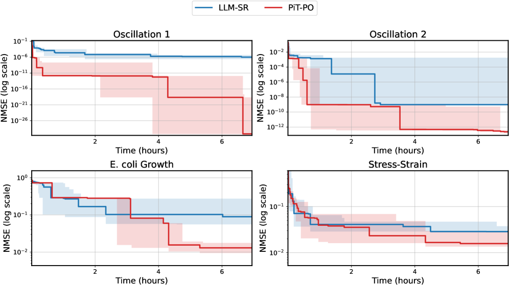
The image displays a 2x2 grid of four line charts comparing the performance of two methods, **LLM-SR** (blue line) and **PiT-PO** (red line), across four different scientific or engineering tasks. Performance is measured by **Normalized Mean Squared Error (NMSE)** on a logarithmic scale over a period of **Time (hours)**. Each chart includes shaded regions around the main lines, indicating variability or confidence intervals.
### Components/Axes
* **Legend:** Located at the top center of the entire figure. It defines:
* **Blue Line:** LLM-SR
* **Red Line:** PiT-PO
* **Common Axes:**
* **X-axis (All Charts):** Label: `Time (hours)`. Scale: Linear, from 0 to approximately 7 hours. Major tick marks at 0, 2, 4, 6.
* **Y-axis (All Charts):** Label: `NMSE (log scale)`. Scale: Logarithmic (base 10). The range varies per subplot.
* **Subplot Titles (Top Center of each panel):**
1. **Top-Left:** `Oscillation 1`
2. **Top-Right:** `Oscillation 2`
3. **Bottom-Left:** `E. coli Growth`
4. **Bottom-Right:** `Stress-Strain`
### Detailed Analysis
**1. Oscillation 1 (Top-Left Panel)**
* **Y-axis Range:** 10⁻¹ to 10⁻²⁶ (a very wide range).
* **LLM-SR (Blue):** Starts near 10⁻¹ at t=0. Shows a stepwise decrease, plateauing around 10⁻⁶ after ~1 hour and remaining relatively flat until the end (~7 hours). The shaded blue region is narrow.
* **PiT-PO (Red):** Starts significantly lower, near 10⁻⁶ at t=0. Exhibits a dramatic, multi-step decline. Major drops occur around t=0.5h, t=4h, and t=6.5h, reaching an extremely low NMSE of approximately 10⁻²⁶ by the end. The shaded red region is very wide, especially after t=2h, indicating high variance in the lower error range.
**2. Oscillation 2 (Top-Right Panel)**
* **Y-axis Range:** 10⁻² to 10⁻¹².
* **LLM-SR (Blue):** Starts near 10⁻². Drops sharply to ~10⁻⁵ within the first hour, then to ~10⁻⁹ around t=3h, where it plateaus. The shaded blue region is moderately wide.
* **PiT-PO (Red):** Starts near 10⁻³. Drops very rapidly to ~10⁻⁹ within the first hour. It continues a stepwise decline, reaching approximately 10⁻¹² by t=7h. The shaded red region is wide, overlapping with the blue region initially but extending to lower values later.
**3. E. coli Growth (Bottom-Left Panel)**
* **Y-axis Range:** 10⁰ (1) to 10⁻².
* **LLM-SR (Blue):** Starts near 10⁰. Shows a gradual, stepwise decline, ending near 10⁻¹. The shaded blue region is consistently wide.
* **PiT-PO (Red):** Starts near 10⁰, similar to LLM-SR. Follows a similar initial trajectory but begins to diverge downward after t=2h. It shows a more pronounced step around t=4.5h, ending near 10⁻². The shaded red region is also wide, generally positioned below the blue region after t=3h.
**4. Stress-Strain (Bottom-Right Panel)**
* **Y-axis Range:** 10⁻¹ to 10⁻².
* **LLM-SR (Blue):** Starts near 10⁻¹. Declines in steps, plateauing around 3x10⁻² after t=4h. The shaded blue region is moderately wide.
* **PiT-PO (Red):** Starts near 10⁻¹. Follows a very similar stepwise decline pattern to LLM-SR but consistently achieves a slightly lower NMSE at each plateau. It ends just above 10⁻². The shaded red region is wide and largely overlaps with the blue region, though its central tendency is slightly lower.
### Key Observations
1. **Consistent Superiority of PiT-PO:** In all four tasks, the PiT-PO method (red) achieves a lower final NMSE than the LLM-SR method (blue).
2. **Magnitude of Improvement:** The performance gap is most extreme in the oscillation tasks. In "Oscillation 1," PiT-PO reaches an error ~20 orders of magnitude lower than LLM-SR. The gap is smallest in the "Stress-Strain" task.
3. **Stepwise Convergence:** Both methods exhibit a characteristic "stepwise" decrease in error, suggesting discrete improvements or optimization phases rather than a smooth, continuous convergence.
4. **Variability:** The shaded confidence intervals for PiT-PO are generally wider than those for LLM-SR, particularly in the oscillation tasks where its performance is best. This indicates higher variance in its results, even as its median/mean performance is superior.
5. **Task Dependency:** The initial error and the rate of convergence are highly dependent on the task. "Oscillation 1" shows the most dramatic improvement, while "Stress-Strain" shows the most modest gains for PiT-PO over LLM-SR.
### Interpretation
The data strongly suggests that the **PiT-PO method is more effective than LLM-SR at minimizing model error over time** for the tested dynamical systems and growth models. Its advantage is particularly pronounced in systems characterized by oscillations ("Oscillation 1" & "2"), where it achieves astronomically lower error values.
The stepwise nature of the error reduction implies that both algorithms may operate in distinct phases—perhaps alternating between exploration and exploitation, or undergoing periodic model updates. The wider confidence intervals for PiT-PO could mean its performance is more sensitive to initial conditions or random seeds, but its central tendency is decisively better.
From a practical standpoint, if the goal is to achieve the highest possible accuracy (lowest NMSE) given sufficient computational time (several hours), **PiT-PO appears to be the superior choice**, especially for oscillatory problems. However, the higher variance might be a consideration for applications requiring highly consistent, predictable performance. The "Stress-Strain" result indicates that for some problem types, the advantage of PiT-PO, while present, may be marginal.