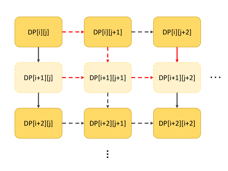
## Diagram: Dynamic Programming Dependency Graph ### Overview The image depicts a dependency graph, likely representing a dynamic programming approach. It shows the relationships between different states or subproblems, denoted as DP[i][j], DP[i][j+1], etc. The arrows indicate the dependencies, with different arrow styles (solid, dashed, red dashed) possibly representing different types or strengths of dependencies. The diagram illustrates how the solution to a particular state depends on the solutions to other states. ### Components/Axes * **Nodes:** Each node is a rounded rectangle labeled as DP[i][j], DP[i][j+1], DP[i][j+2], DP[i+1][j], DP[i+1][j+1], DP[i+1][j+2], DP[i+2][j], DP[i+2][j+1], DP[i+2][j+2]. The nodes in the first and third rows are solid yellow, while the nodes in the second row are dashed yellow. * **Edges:** The edges are represented by arrows, indicating the direction of dependency. There are three types of arrows: * Solid black arrows pointing downwards. * Dashed black arrows pointing to the right or downwards. * Dashed red arrows pointing to the right or downwards. * **Ellipsis:** Two sets of ellipsis (...) indicate that the pattern continues beyond what is shown in the diagram. One is on the right side of the second row, and the other is below the third row. ### Detailed Analysis or Content Details * **Row 1:** * Node 1: DP[i][j] (solid yellow) * Node 2: DP[i][j+1] (solid yellow) * Node 3: DP[i][j+2] (solid yellow) * Dependencies: DP[i][j] -> DP[i][j+1] (red dashed arrow), DP[i][j+1] -> DP[i][j+2] (dashed arrow) * **Row 2:** * Node 4: DP[i+1][j] (dashed yellow) * Node 5: DP[i+1][j+1] (dashed yellow) * Node 6: DP[i+1][j+2] (dashed yellow) * Dependencies: DP[i+1][j] -> DP[i+1][j+1] (red dashed arrow), DP[i+1][j+1] -> DP[i+1][j+2] (red dashed arrow) * **Row 3:** * Node 7: DP[i+2][j] (solid yellow) * Node 8: DP[i+2][j+1] (solid yellow) * Node 9: DP[i+2][j+2] (solid yellow) * Dependencies: DP[i+2][j] -> DP[i+2][j+1] (dashed arrow), DP[i+2][j+1] -> DP[i+2][j+2] (dashed arrow) * **Column 1:** * Dependencies: DP[i][j] -> DP[i+1][j] (solid arrow), DP[i+1][j] -> DP[i+2][j] (solid arrow) * **Column 2:** * Dependencies: DP[i][j+1] -> DP[i+1][j+1] (red dashed arrow), DP[i+1][j+1] -> DP[i+2][j+1] (dashed arrow) * **Column 3:** * Dependencies: DP[i][j+2] -> DP[i+1][j+2] (red dashed arrow), DP[i+1][j+2] -> DP[i+2][j+2] (solid arrow) ### Key Observations * The diagram represents a 2D grid of states, indexed by `i` and `j`. * Dependencies exist both horizontally (within the same row) and vertically (within the same column). * The arrow styles (solid, dashed, red dashed) suggest different types or strengths of dependencies. * The dashed nodes in the second row might indicate intermediate or optional states. * The ellipsis indicate that the pattern continues indefinitely in both horizontal and vertical directions. ### Interpretation The diagram illustrates a typical dependency structure found in dynamic programming problems. The states DP[i][j] represent subproblems, and the arrows indicate which subproblems need to be solved before a particular subproblem can be solved. The different arrow styles could represent different costs or probabilities associated with the dependencies. The dashed nodes might represent states that are only conditionally required, or states that are computed differently. The diagram provides a visual representation of the order in which the subproblems need to be solved to arrive at the final solution. The specific meaning of 'i' and 'j' would depend on the particular dynamic programming problem being represented.

\n ## Diagram: Dynamic Programming State Transition ### Overview The image depicts a diagram illustrating a state transition process, likely related to dynamic programming. It shows a grid-like structure of interconnected nodes labeled with `DP[i][j]` and its variations, connected by arrows indicating dependencies. The diagram suggests a recursive or iterative calculation where the value of a state depends on the values of previous states. ### Components/Axes The diagram consists of rectangular nodes, each labeled with `DP[i][j]` where `i` and `j` are indices. The arrows represent transitions between states. There are no explicit axes or scales. The diagram extends downwards and to the right, indicated by the ellipsis (`...`). ### Detailed Analysis or Content Details The diagram shows a 3x3 grid of `DP` states, with an indication that this pattern continues. The nodes are arranged as follows: * **Top Row:** `DP[i][j]`, `DP[i][j+1]`, `DP[i][j+2]` * **Middle Row:** `DP[i+1][j]`, `DP[i+1][j+1]`, `DP[i+1][j+2]` * **Bottom Row:** `DP[i+2][j]`, `DP[i+2][j+1]`, `DP[i+2][j+2]` The arrows indicate the following dependencies: * `DP[i][j]` -> `DP[i][j+1]` (solid red arrow) * `DP[i][j+1]` -> `DP[i][j+2]` (dashed red arrow) * `DP[i][j]` -> `DP[i+1][j]` (solid yellow arrow) * `DP[i+1][j]` -> `DP[i+2][j]` (solid yellow arrow) * `DP[i][j+1]` -> `DP[i+1][j+1]` (dashed yellow arrow) * `DP[i+1][j+1]` -> `DP[i+2][j+1]` (dashed yellow arrow) * `DP[i][j+2]` -> `DP[i+1][j+2]` (solid red arrow) * `DP[i+1][j+2]` -> `DP[i+2][j+2]` (solid red arrow) The diagram shows a pattern of dependencies where each state `DP[i][j]` depends on states in the same row and the row above. The solid arrows represent a stronger dependency, while the dashed arrows represent a weaker or different type of dependency. ### Key Observations The diagram illustrates a dynamic programming approach where the solution to a problem is built up from solutions to subproblems. The indices `i` and `j` likely represent dimensions or stages in the problem. The use of both solid and dashed arrows suggests different types of transitions or dependencies between states. The ellipsis indicates that the grid extends indefinitely, implying a potentially large state space. ### Interpretation This diagram likely represents a state transition diagram for a dynamic programming algorithm. The `DP[i][j]` notation suggests that the algorithm is storing intermediate results in a table or matrix. The arrows indicate how the value of a state `DP[i][j]` is calculated based on the values of other states. The solid and dashed arrows could represent different costs or weights associated with the transitions. The diagram suggests that the problem being solved can be broken down into smaller, overlapping subproblems. The dynamic programming approach allows the algorithm to avoid redundant calculations by storing the solutions to subproblems and reusing them when needed. The pattern of dependencies indicates that the algorithm is likely solving a problem with a grid-like structure, such as a pathfinding problem or a matrix optimization problem. The diagram does not provide specific data or numerical values, but it illustrates the general structure of a dynamic programming solution.

## Diagram: Data Processing Node Network ### Overview The diagram illustrates a structured network of data processing nodes arranged in a grid pattern. Nodes are labeled with DP[i][j] notation, where "i" and "j" represent row and column indices. Arrows indicate directional relationships between nodes, with distinct styling for horizontal vs vertical connections. The middle row of nodes is visually emphasized through background highlighting. ### Components/Axes - **Nodes**: - Labeled using DP[i][j] syntax (e.g., DP[1][1], DP[2][3]) - Organized in a 3x3 grid structure (visible portion) - Color-coded: - Top/bottom rows: Yellow background - Middle row: Light yellow background - **Arrows**: - Horizontal connections: Dashed red arrows (left-to-right flow) - Vertical connections: Solid black arrows (top-to-bottom flow) - **Special Elements**: - Middle row nodes highlighted with light yellow background - Ellipsis (...) indicates continuation beyond visible grid ### Detailed Analysis 1. **Node Relationships**: - Horizontal flow: DP[i][j] → DP[i][j+1] → DP[i][j+2] (dashed red) - Vertical flow: DP[i][j] → DP[i+1][j] → DP[i+2][j] (solid black) - Diagonal relationships implied through combined flows 2. **Indexing Pattern**: - Row index "i" increments downward (top=1, middle=2, bottom=3) - Column index "j" increments rightward (left=1, center=2, right=3) 3. **Highlighted Middle Row**: - DP[2][j] nodes emphasized through background color - Suggests special processing layer or priority status ### Key Observations 1. Structured grid organization enables systematic data flow 2. Dual-directional connectivity allows both row-wise and column-wise processing 3. Middle row emphasis implies potential bottleneck or critical processing stage 4. Consistent labeling convention supports scalable network expansion ### Interpretation This diagram represents a multi-stage data processing pipeline where: 1. **Horizontal Flow** (dashed red): Represents sequential processing within the same row (e.g., feature extraction stages) 2. **Vertical Flow** (solid black): Indicates data aggregation or transformation between processing layers 3. **Middle Row Emphasis**: Suggests this layer might contain: - Core processing logic - Data validation checkpoint - Resource-intensive operations 4. The grid structure enables: - Parallel processing capabilities - Modular system design - Scalable architecture through index-based addressing The network's design implies a balance between horizontal data propagation and vertical transformation, with the middle row serving as a critical integration point. The consistent labeling convention and directional arrows create a self-documenting system that could be extended to larger dimensions while maintaining operational clarity.