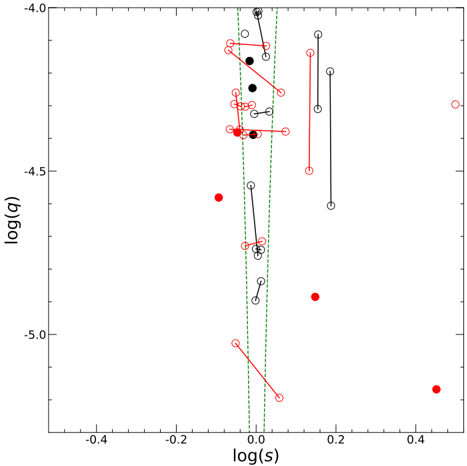
## Scatter Plot: Log-Log Comparison of Model A and Model B ### Overview The image is a log-log scatter plot comparing two models (Model A and Model B) across variables `s` (x-axis) and `q` (y-axis). The plot includes reference lines at `log(s) = 0` (green dashed vertical line) and `log(q) = -4.5` (green dashed horizontal line). Data points are color-coded: red for Model A and black for Model B, with connecting lines indicating relationships between points. --- ### Components/Axes - **X-axis (log(s))**: Ranges from -0.4 to 0.4, labeled "log(s)". - **Y-axis (log(q))**: Ranges from -5.0 to -4.0, labeled "log(q)". - **Legend**: - Red: Model A - Black: Model B - **Reference Lines**: - Green dashed vertical line at `log(s) = 0`. - Green dashed horizontal line at `log(q) = -4.5`. --- ### Detailed Analysis #### Model A (Red Points) - **Data Points**: 1. (-0.3, -4.8) 2. (-0.1, -4.6) 3. (0.1, -4.7) 4. (0.2, -4.5) 5. (0.3, -4.4) 6. (0.4, -5.0) - **Trend**: Points are scattered but show a slight upward trend as `log(s)` increases. A connecting line links (-0.3, -4.8) → (-0.1, -4.6) → (0.1, -4.7) → (0.2, -4.5) → (0.3, -4.4), suggesting a gradual increase in `log(q)` with `log(s)`. #### Model B (Black Points) - **Data Points**: 1. (-0.2, -4.3) 2. (0.0, -4.5) 3. (0.1, -4.6) 4. (0.2, -4.4) 5. (0.3, -4.3) - **Trend**: Points cluster tightly around `log(s) = 0` and `log(q) = -4.5`. A connecting line links (-0.2, -4.3) → (0.0, -4.5) → (0.1, -4.6) → (0.2, -4.4) → (0.3, -4.3), indicating minimal variation in `log(q)` across `log(s)`. #### Reference Lines - **Vertical Line (log(s) = 0)**: Separates negative and positive `s` values. Model B’s points are concentrated near this line. - **Horizontal Line (log(q) = -4.5)**: Model B’s points align closely with this line, while Model A’s points deviate slightly. --- ### Key Observations 1. **Model A**: - Higher variability in `log(q)` values (range: -5.0 to -4.4). - Outlier at (0.4, -5.0), significantly lower than other points. - Connecting lines suggest a weak positive correlation between `log(s)` and `log(q)`. 2. **Model B**: - Tighter clustering around `log(s) = 0` and `log(q) = -4.5`. - Minimal variation in `log(q)` (range: -4.6 to -4.3). - Points align with the reference lines, indicating stability. 3. **Reference Lines**: - Model B’s data is tightly bound to the green lines, while Model A’s data spreads beyond them. --- ### Interpretation - **Model Performance**: Model B demonstrates greater consistency and stability, with data points tightly clustered near the reference lines. This suggests it may be more reliable or efficient for the measured variables. - **Model A**: Exhibits higher variability, with an outlier at (0.4, -5.0) that could indicate edge-case behavior or measurement noise. The weak upward trend might imply sensitivity to changes in `s`. - **Reference Lines**: The green lines likely represent critical thresholds or baseline values. Model B’s alignment with these lines suggests it operates within expected ranges, while Model A’s deviations may require further investigation. This analysis highlights trade-offs between Model A’s variability and Model B’s stability, guiding decisions on which model to prioritize based on the application’s requirements for precision or adaptability.