## Multi-Chart: Array Relaxation and MVM Simulations ### Overview The image presents a series of six charts (a-f) that analyze the relaxation behavior of a programmed array and its impact on hardware-aware Matrix-Vector Multiplication (MVM) simulations. The charts cover aspects like probability density of programmed conductance, standard deviation of conductance relaxation, G-state relaxation over time, relaxation error, extended array relaxation at a specific conductance, and the performance of MVM simulations. ### Components/Axes **Chart a: Array relaxation after 10min** * **Title:** Array relaxation after 10min * **Y-axis:** Probability Density, Scale: 0.00 to 1.00, incremented by 0.25 * **X-axis:** Programmed Conductance [µS], Scale: 10 to 90, incremented by 10 * **Annotation:** Adjacent State Gaussian Overlap (10min): 9.6% * **Color Gradient:** The bars are colored in a gradient from blue (left) to red (right), corresponding to lower and higher programmed conductance values. * **States:** A secondary y-axis on the right side, ranging from 1 to 35. **Chart b: Std. dev. conductance relaxation** * **Title:** Std. dev. conductance relaxation * **Y-axis:** Standard deviation [µS], Scale: 0.0 to 1.0, incremented by 0.2 * **X-axis:** Programmed Conductance [µS], Scale: 10 to 90, incremented by 10 * **Legend:** * Blue-purple circles: During Programming (Acc. Range 0.2%) * Light blue circles: 10 min After Programming * **Annotation:** "Array Relaxation After 10 min" with arrows pointing to the respective data series. **Chart c: G-state relaxation after 1h** * **Title:** G-state relaxation after 1h * **Y-axis:** Programmed Conductance [µS], Scale: 10 to 90, incremented by 10 * **X-axis:** Time after programming [s], Logarithmic scale from 10^0 to 10^3 * **Color Gradient:** The lines are colored in a gradient from blue (bottom) to red (top), corresponding to lower and higher programmed conductance values. **Chart d: 1h-relaxation error** * **Title:** 1h-relaxation error * **Y-axis:** G1h - Gprog. [µS], Scale: -3 to 3, incremented by 1 * **X-axis:** Programmed Conductance [µS], Scale: 10 to 90, incremented by 10 * **Annotation:** Avg. 1h-Relaxation Error = -0.68 µS (dashed black line) * **Color Gradient:** The data points are colored in a gradient from blue (left) to red (right), corresponding to lower and higher programmed conductance values. **Chart e: Extended array relaxation at 50µS** * **Title:** Extended array relaxation at 50µS * **Main Plot:** * **Y-axis:** Normalized Probability Density, Scale: 0.00 to 1.00, incremented by 0.25 * **X-axis:** Programmed Conductance [µS], Scale: 40 to 60, incremented by 5 * **Legend:** * Dark Blue: Prog. * Light Blue: 1s * Orange: 1h * Light Red: 1d * Red: 2d * Purple: 1w * Dashed Black: 10y * **Inset Plot 1 (top-right):** * **Y-axis:** Mean [µS], Scale: 45 to 50, incremented by 5 * **X-axis:** Log(Time[s]), Scale: 0 to 20, incremented by 10 * **Data Points:** Prog, 1s, 1h, 1d, 10y * **Inset Plot 2 (bottom-right):** * **Y-axis:** Std Dev. [µS], Scale: 0 to 1, incremented by 1 * **X-axis:** Log(Time[s]), Scale: 0 to 20, incremented by 10 * **Data Points:** Prog, 1s, 1h, 1d, 10y **Chart f: HW-aware MVM simulations** * **Title:** HW-aware MVM simulations * **Y-axis:** ReRAM inner product output * **X-axis:** Expected inner product output * **Legend:** * Blue: Prog * Light Blue: 1s * Orange: 1h * Light Red: 1d * Black: 10y * Red: ideal * **Annotation:** 64x64 Forward MVM, 6b input, 8b output * **Inset Plot:** * **Y-axis:** RMSE * **X-axis:** Log(Time[s]), Scale: 0 to 20, incremented by 10 * **Data Points:** Prog, 1s, 1h, 1d, 10y ### Detailed Analysis **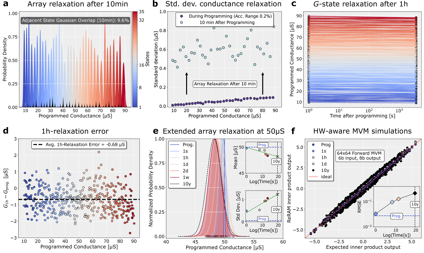Chart a:** Shows the probability density of programmed conductance states after 10 minutes. The distribution appears multimodal, with peaks at various conductance levels. The color gradient indicates the programmed conductance value, with blue representing lower values and red representing higher values. The Adjacent State Gaussian Overlap is 9.6%, indicating the degree of overlap between adjacent conductance states. **Chart b:** Illustrates the standard deviation of conductance relaxation. The "During Programming" data series shows very low standard deviation values, close to zero, across all programmed conductance levels. The "10 min After Programming" data series shows a higher standard deviation, fluctuating between approximately 0.4 and 0.8 µS. **Chart c:** Depicts the G-state relaxation over time. Each line represents a different programmed conductance level, and the x-axis shows the time after programming on a logarithmic scale. The conductance values appear to decrease slightly over time, with the higher conductance states (red lines) showing a more pronounced decrease. **Chart d:** Shows the 1-hour relaxation error (G1h - Gprog) as a function of programmed conductance. The data points are scattered around the zero line, with some points above and some below. The average 1-hour relaxation error is -0.68 µS, indicated by the dashed black line. **Chart e:** Focuses on the extended array relaxation at 50 µS. The main plot shows the normalized probability density of the conductance at different time points (Prog, 1s, 1h, 1d, 2d, 1w, 10y). The inset plots show the mean and standard deviation of the conductance as a function of the logarithm of time. Both the mean and standard deviation decrease over time. * **Main Plot:** The "Prog." (programmed) distribution is the narrowest, indicating the initial state. As time increases (1s, 1h, 1d, 2d, 1w), the distributions broaden, and the peak shifts slightly to the left. The "10y" (10 years) distribution is the broadest and most shifted. * **Inset Plot 1 (Mean vs. Log(Time)):** The mean conductance decreases approximately linearly with the logarithm of time. The data points are: * Prog: ~50 µS at Log(Time) = 0 * 1s: ~49.5 µS at Log(Time) ~ 0 * 1h: ~49 µS at Log(Time) ~ 3.6 * 1d: ~48.5 µS at Log(Time) ~ 4.6 * 10y: ~46 µS at Log(Time) ~ 8 * **Inset Plot 2 (Std Dev vs. Log(Time)):** The standard deviation also decreases approximately linearly with the logarithm of time. * Prog: ~0.5 µS at Log(Time) = 0 * 1s: ~0.5 µS at Log(Time) ~ 0 * 1h: ~0.4 µS at Log(Time) ~ 3.6 * 1d: ~0.3 µS at Log(Time) ~ 4.6 * 10y: ~0.2 µS at Log(Time) ~ 8 **Chart f:** Presents the results of hardware-aware MVM simulations. The main plot shows the ReRAM inner product output versus the expected inner product output. The data points for different time points (Prog, 1s, 1h, 1d, 10y) are clustered closely around the "ideal" line, indicating good agreement between the ReRAM output and the expected output. The inset plot shows the Root Mean Square Error (RMSE) as a function of the logarithm of time. The RMSE increases over time, indicating a degradation in performance due to relaxation. * **Main Plot:** The data points are tightly clustered around the ideal line, indicating high accuracy in the MVM operation. * **Inset Plot (RMSE vs. Log(Time)):** The RMSE increases approximately linearly with the logarithm of time. * Prog: ~0.01 at Log(Time) = 0 * 1s: ~0.01 at Log(Time) ~ 0 * 1h: ~0.02 at Log(Time) ~ 3.6 * 1d: ~0.03 at Log(Time) ~ 4.6 * 10y: ~0.1 at Log(Time) ~ 8 ### Key Observations * **Conductance Relaxation:** The programmed conductance values tend to decrease over time (Chart c and e). * **Increased Variability:** The standard deviation of conductance increases shortly after programming (Chart b) but decreases over longer periods (Chart e). * **Performance Degradation:** The accuracy of MVM simulations degrades over time due to conductance relaxation (Chart f). * **Error Distribution:** The 1-hour relaxation error is centered around -0.68 µS (Chart d). ### Interpretation The data suggests that conductance relaxation is a significant factor affecting the long-term stability and performance of ReRAM-based systems. While the initial programming accuracy is high, the conductance values drift over time, leading to increased variability and reduced accuracy in MVM operations. The extended array relaxation analysis at 50 µS (Chart e) provides insights into the temporal dynamics of this relaxation process, showing that both the mean and standard deviation of the conductance decrease over time. The hardware-aware MVM simulations (Chart f) demonstrate that this relaxation-induced drift can degrade the performance of neural network computations. The results highlight the need for strategies to mitigate the effects of conductance relaxation in ReRAM-based systems, such as periodic reprogramming or error correction techniques. The adjacent state Gaussian overlap of 9.6% indicates that the programmed states are relatively well-separated, but the relaxation process can cause these states to drift and potentially overlap, further degrading performance.

\n ## Charts/Graphs: Array Relaxation and Hardware-Aware MVM Simulations ### Overview The image presents six charts (a-f) detailing the relaxation behavior of an array after programming, and simulations of hardware-aware Matrix-Vector Multiplication (MVM). The charts explore conductance relaxation over various timescales (10 minutes, 1 hour, 50 microseconds, and up to 1 week), standard deviation of conductance, and the performance of MVM simulations. ### Components/Axes * **a) Array relaxation after 10min:** * X-axis: Programmed Conductance \[µS] (Scale: 0 to 90, increments of 10) * Y-axis: Probability Density (Scale: 0 to 1.0, increments of 0.25) * Title: "Array relaxation after 10min" * Annotation: "Adjacent Gaussian Overlay (10min): 9.6%" * **b) Std. dev. conductance relaxation:** * X-axis: Programmed Conductance \[µS] (Scale: 0 to 90, increments of 10) * Y-axis: Standard deviation \[µS] (Scale: 0 to 32, increments of 8) * Title: "Std. dev. conductance relaxation" * Legend: * Green circles: "During Programming (Acc. Range 0.2%)" * Black circles: "10 min After Programming" * Annotation: "Array Relaxation After 10 min" with an arrow pointing to the data. * **c) G-state relaxation after 1h:** * X-axis: Time after programming \[s] (Logarithmic scale: 10⁰ to 10³, increments are not clearly marked) * Y-axis: Programmed Conductance \[µS] (Scale: 0 to 90, increments of 20) * Title: "G-state relaxation after 1h" * **d) 1h-relaxation error:** * X-axis: Programmed Conductance \[µS] (Scale: 0 to 90, increments of 10) * Y-axis: G_fin - G_prog \[µS] (Scale: -3 to 3, increments of 1) * Title: "1h-relaxation error" * Annotation: "Avg. 1h-Relaxation Error = -0.68 µS" * **e) Extended array relaxation at 50µs:** * X-axis: Programmed Conductance \[µS] (Scale: 0 to 60, increments of 10) * Y-axis: Normalized Probability Density (Scale: 0 to 1.0, increments of 0.25) * Title: "Extended array relaxation at 50µs" * Legend: * Prog.: Solid line * 1s: Dashed line * 1d: Dotted line * 2d: Dashed-dotted line * 1w: Long dashed-dotted line * Inset Chart: * X-axis: Log(Time[s]) * Y-axis: Mean \[µS] (Top) and Std Dev. \[µS] (Bottom) * **f) HW-aware MVM simulations:** * X-axis: Expected inner product output (Scale: -5 to 2.5, increments of 1) * Y-axis: ReRAM inner product output (Scale: 0 to 5, increments of 1) * Title: "HW-aware MVM simulations" * Annotation: "64x64 Forward MVM, 6b input, 8b output" * Legend: * Prog.: Solid line * 1s: Dashed line * 1h: Dotted line * 1d: Dashed-dotted line * 10y: Long dashed-dotted line * Inset Chart: * X-axis: Log(Time[s]) * Y-axis: RMSE (Logarithmic scale: 10⁻¹ to 10⁰, increments of 0.2) ### Detailed Analysis or Content Details * **a)** The probability density distribution shows a peak around 30-40 µS, with a tail extending towards higher conductance values. The adjacent Gaussian overlay suggests a 9.6% overlap. * **b)** The standard deviation of conductance is relatively stable during programming (green circles), with values ranging from approximately 2 to 8 µS. After 10 minutes, the standard deviation increases slightly, with values ranging from approximately 4 to 12 µS. * **c)** The programmed conductance decreases over time after programming, with a rapid initial drop followed by a slower decay. At t=1s, conductance is approximately 80 µS, decreasing to approximately 40 µS at t=100s, and leveling off around 30 µS at t=1000s. * **d)** The 1h-relaxation error (G_fin - G_prog) is generally negative, indicating that the final conductance is lower than the programmed conductance. The average 1h-relaxation error is -0.68 µS. The data points are scattered around the zero line, with a slight concentration of points below the line. * **e)** The normalized probability density distribution shifts towards lower conductance values as time increases. At Prog., the peak is around 40 µS. After 1s, the peak shifts to approximately 35 µS. After 1 week (1w), the peak shifts further to approximately 30 µS. The inset chart shows that the mean conductance decreases over time, while the standard deviation remains relatively constant. * **f)** The ReRAM inner product output closely follows the expected inner product output, especially for shorter times (Prog., 1s, 1h). As time increases (1d, 10y), the ReRAM output deviates from the expected output. The RMSE increases with time, indicating a decrease in accuracy. The RMSE is approximately 0.01 at Prog., increasing to approximately 0.1 at 10y. ### Key Observations * Conductance relaxation is a significant phenomenon, with conductance decreasing over time after programming. * The standard deviation of conductance increases slightly after relaxation. * The 1h-relaxation error is consistently negative, suggesting a systematic underestimation of the final conductance. * MVM simulations show good accuracy for short times, but accuracy degrades over time due to conductance drift. * The inset charts in (e) and (f) provide a more detailed view of the trends observed in the main charts. ### Interpretation The data suggests that the ReRAM array exhibits conductance relaxation, which is a critical factor to consider for long-term reliability and accuracy. The relaxation process leads to a decrease in conductance over time, which can affect the performance of MVM operations. The simulations in (f) demonstrate that the accuracy of MVM operations degrades as the conductance drifts, highlighting the need for calibration or compensation techniques to mitigate the effects of relaxation. The adjacent Gaussian overlay in (a) suggests that the relaxation process is not uniform across the array, and that some devices may relax more quickly than others. The consistent negative relaxation error in (d) indicates a systematic bias in the relaxation process, which could be due to device-specific characteristics or programming conditions. The logarithmic scales used in (c) and (f) emphasize the importance of long-term stability and the potential for significant degradation over extended periods. Overall, the data provides valuable insights into the behavior of ReRAM arrays and the challenges associated with implementing reliable and accurate MVM operations.

## Multi-Panel Scientific Figure: Conductance Relaxation in Memory Arrays ### Overview This image is a composite scientific figure containing six panels (a-f) that collectively analyze the relaxation (drift or decay) of conductance states in an analog memory array (likely ReRAM or a similar technology) over time. The data explores how programmed conductance values change after programming, the resulting errors, and the impact on hardware-aware matrix-vector multiplication (MVM) simulations. ### Components/Axes The figure is divided into six distinct panels, labeled **a** through **f** in the top-left corner of each subplot. * **Panel a:** Histogram titled "Array relaxation after 10min". * **X-axis:** "Programmed Conductance [µS]" (range: ~10 to 90 µS). * **Y-axis:** "Probability Density" (range: 0.00 to 1.00). * **Color Bar (Right):** Labeled "States", scale from 1 (blue) to 35 (red). * **Annotation:** A text box in the upper left states "Adjacent State Gaussian Overlap (10min): 9.6%". * **Panel b:** Scatter plot titled "Std. dev. conductance relaxation". * **X-axis:** "Programmed Conductance [µS]" (range: 10 to 90 µS). * **Y-axis:** "Standard deviation [µS]" (range: 0.0 to 1.0 µS). * **Legend (Top-Left):** Two entries: "During Programming (Acc. Range 0.2%)" (filled purple circles) and "10 min After Programming" (open light-blue circles). * **Annotation:** Two black arrows point from the "During Programming" data series upward to the "10 min After" series, with a label "Array Relaxation After 10 min". * **Panel c:** Line plot titled "G-state relaxation after 1h". * **X-axis:** "Time after programming [s]" (logarithmic scale, range: 10⁰ to ~10³ seconds). * **Y-axis:** "Programmed Conductance [µS]" (range: 10 to 90 µS). * **Data:** Multiple lines, each representing a single memory cell's conductance over time. Lines are colored on a gradient from blue (low initial conductance) to red (high initial conductance). * **Panel d:** Scatter plot titled "1h-relaxation error". * **X-axis:** "Programmed Conductance [µS]" (range: 10 to 90 µS). * **Y-axis:** "G₁ₕ - G_prog [µS]" (range: -3 to 3 µS). This represents the error after 1 hour. * **Annotation:** A horizontal dashed black line is drawn at y = -0.68 µS. A text box states "Avg. 1h-Relaxation Error = -0.68 µS". * **Data Points:** Colored circles, with color corresponding to the "States" color bar from panel **a** (blue for low states, red for high states). * **Panel e:** Composite plot titled "Extended array relaxation at 50µS". * **Main Plot (Left):** * **X-axis:** "Programmed Conductance [µS]" (range: 40 to 60 µS). * **Y-axis:** "Normalized Probability Density" (range: 0.00 to 1.00). * **Legend:** Seven entries: "Prog.", "1s", "1h", "1d", "2d", "1w", "10y". Each corresponds to a distribution curve at a different time after programming. * **Top Inset (Right):** * **X-axis:** "Log(Time[s])" (range: 0 to 20). * **Y-axis:** "Mean [µS]" (range: 45 to 50 µS). * **Data:** Points showing the mean conductance decaying over log time. A dashed green line connects the "Prog." point to the "10y" point. * **Bottom Inset (Right):** * **X-axis:** "Log(Time[s])" (range: 0 to 20). * **Y-axis:** "Std Dev. [µS]" (range: 0 to 1 µS). * **Data:** Points showing the standard deviation increasing over log time. A dashed green line connects the "Prog." point to the "10y" point. * **Panel f:** Scatter plot titled "HW-aware MVM simulations". * **X-axis:** "Expected inner product output" (range: -5.0 to 5.0). * **Y-axis:** "ReRAM inner product output" (range: -5.0 to 5.0). * **Legend (Top-Left):** Six entries: "Prog", "1s", "1h", "1d", "10y" (different colored circles), and "ideal" (solid red line). * **Annotation:** A text box states "64x64 Forward MVM 6b input, 8b output". * **Inset (Bottom-Right):** * **X-axis:** "Log(Time[s])" (range: 0 to 20). * **Y-axis:** "RMSE" (logarithmic scale, range: 10⁻² to 10⁻¹). * **Data:** Points showing the Root Mean Square Error of the MVM output increasing over log time. A dashed blue line connects the "Prog." point to the "10y" point. ### Detailed Analysis * **Panel a:** The histogram shows the distribution of conductance states across the array 10 minutes after programming. The distribution is multi-modal, with distinct peaks corresponding to the 35 programmed states. The color gradient visually maps the state number (1-35) to the conductance value. The 9.6% Gaussian overlap quantifies the probability of misidentifying adjacent states due to relaxation-induced broadening. * **Panel b:** This plot directly compares the precision of programming. The "During Programming" data (purple) shows very low standard deviation (< ~0.1 µS), indicating tight control. After 10 minutes of relaxation (light blue), the standard deviation increases significantly (to ~0.4-0.8 µS), and this increase is more pronounced for higher programmed conductance values (positive slope in the light blue data). * **Panel c:** This plot visualizes the temporal drift of individual cells. All conductance lines show a downward trend (decay) over the 1-hour period (~3600 seconds). The decay appears more severe (steeper initial slope) for cells programmed to higher conductance values (red lines) compared to lower ones (blue lines). * **Panel d:** The scatter plot shows the error (final - initial conductance) for each cell after 1 hour. The data is scattered around a negative mean (-0.68 µS), indicating a systematic downward drift. The spread (variance) of the error appears relatively consistent across the programmed conductance range, though there may be a slight increase in spread for mid-range conductances. * **Panel e:** This panel focuses on the long-term statistical evolution of a single conductance state (centered at 50 µS). The main plot shows the probability distribution broadening and shifting left (to lower conductance) over time, from "Prog." to "10y". The insets quantify this: the mean conductance decays linearly with log(time), while the standard deviation increases linearly with log(time). This is characteristic of a logarithmic relaxation process. * **Panel f:** This panel assesses the functional impact of relaxation on a computational task (64x64 matrix-vector multiplication). The main plot shows that the actual ReRAM output correlates very strongly with the expected output (data points cluster tightly around the red "ideal" line) for all time points. The inset quantifies the degradation: the RMSE of the computation increases with log(time), but remains below 0.1 even after a simulated 10 years. ### Key Observations 1. **Systematic Negative Drift:** Conductance states consistently decay over time, with an average 1-hour error of -0.68 µS (Panel d). 2. **Increased Variability:** Relaxation not only shifts the mean but also increases the standard deviation (spread) of conductance values (Panels b, e). 3. **Logarithmic Time Dependence:** Both the mean decay and the increase in standard deviation follow a linear relationship with the logarithm of time (Panel e insets). 4. **State-Dependent Effects:** Higher conductance states exhibit greater absolute standard deviation after relaxation (Panel b) and potentially faster initial decay (Panel c). 5. **Robustness in Computation:** Despite significant analog drift at the device level, the system-level performance (MVM accuracy) degrades gracefully, with RMSE increasing only moderately over a simulated decade (Panel f). ### Interpretation This figure presents a comprehensive characterization of conductance drift in an analog memory array, a critical challenge for neuromorphic computing and analog AI hardware. The data demonstrates that while individual devices undergo significant and predictable relaxation following a logarithmic law (Panels c, e), the collective behavior of a large array can be statistically modeled (Panels a, b, d). The key insight is the translation from device-level physics to system-level functionality. The "Adjacent State Gaussian Overlap" (9.6%) is a crucial metric for determining the feasibility of multi-level cell storage. Most importantly, Panel f provides a hardware-aware simulation that bridges this gap, showing that the inherent redundancy and error tolerance in neural network computations (like MVM) can mitigate the effects of analog drift. The system maintains functional accuracy even as individual components degrade, which is a promising result for the long-term reliability of analog AI accelerators. The outlier in Panel d (a point near -3 µS error) suggests occasional catastrophic failure or measurement error in single cells, which would need to be addressed through error correction or circuit design.

## Array Relaxation and Conductance Analysis ### Overview The image presents six panels (a-f) analyzing array relaxation dynamics, conductance stability, and simulation accuracy in resistive memory devices. Panels a-e focus on experimental data, while panel f presents simulation results. Key themes include temporal relaxation behavior, error quantification, and long-term stability. ### Components/Axes **Panel a**: - **X-axis**: Programmed Conductance [µS] (10-90 µS) - **Y-axis**: Probability Density (0-1.0) - **Legend**: Adjacent State Gaussian Overlap (10min): 9.6% - **Color Gradient**: Blue (low) → Red (high) probability density **Panel b**: - **X-axis**: Programmed Conductance [µS] (10-90 µS) - **Y-axis**: Standard Deviation [µS] (0-1.0) - **Markers**: - Purple circles: During Programming (Acc. Range 0.2%) - Green circles: 10 min After Programming - **Annotations**: Arrows labeled "Array Relaxation After 10 min" **Panel c**: - **X-axis**: Time after Programming [s] (log scale: 10⁰-10³) - **Y-axis**: Programmed Conductance [µS] (10-90 µS) - **Color Gradient**: Red (high G-state) → Blue (low G-state) **Panel d**: - **X-axis**: Programmed Conductance [µS] (10-90 µS) - **Y-axis**: 1h-Relaxation Error [G₁h - G_prog] [µS] (-3 to +3) - **Trendline**: Dashed black line (Avg. Error = -0.68 µS) **Panel e**: - **X-axis**: Programmed Conductance [µS] (40-60 µS) - **Y-axis**: Normalized Probability Density (0-1.0) - **Legend**: Time Intervals (1s, 1h, 1d, 1w, 10y) - **Inset Graphs**: - Top: Mean vs. Log(Time) [10y marker at 45 µS] - Bottom: Std. Dev. vs. Log(Time) [10y marker at 55 µS] **Panel f**: - **X-axis**: Expected Inner Product Output (-5 to +5) - **Y-axis**: ReRAM Inner Product Output (-5 to +5) - **Markers**: - Purple circles: Program (Prog) - Blue squares: 1s - Green diamonds: 1h - Red triangles: 10y - **Trendline**: Red dashed line (Ideal 1:1 correlation) - **Inset Graph**: RMSE vs. Log(Time) [10y marker at 10⁻¹ RMSE] ### Detailed Analysis **Panel a**: - Probability density peaks at ~45 µS (blue) and ~75 µS (red), indicating bimodal distribution. - Adjacent state overlap (9.6%) suggests partial conductance state interference. **Panel b**: - Standard deviation decreases by ~0.4 µS after 10 min (green markers vs. purple). - Lower conductance states (<30 µS) show larger relaxation effects. **Panel c**: - G-state relaxation follows exponential decay: - 90 µS → 70 µS in 1s - Stabilizes near 50 µS after 1h. **Panel d**: - Negative average error (-0.68 µS) indicates systematic underestimation of G₁h. - Errors cluster around ±1 µS for mid-range conductances (40-60 µS). **Panel e**: - Conductance stabilizes at ~50 µS after 10y (dashed black line). - Insets show: - Mean shifts from 45 µS (1s) to 55 µS (10y) - Std. Dev. decreases from 5 µS (1s) to 2 µS (10y) **Panel f**: - Strong linear correlation (R² > 0.95) between expected and observed outputs. - 10y data points deviate by <0.5 units from ideal line. - RMSE improves from 0.1 (1s) to 0.01 (10y). ### Key Observations 1. **Temporal Relaxation**: Conductance states relax toward ~50 µS across all time scales (panels a, c, e). 2. **Error Patterns**: Systematic underestimation (-0.68 µS avg.) suggests calibration requirements (panel d). 3. **Simulation Accuracy**: MVM models achieve <1% error after 10y (panel f). 4. **Bimodal Distribution**: Two dominant conductance states emerge post-programming (panel a). ### Interpretation The data demonstrates that resistive memory arrays exhibit predictable relaxation toward a stable conductance state (~50 µS) over time, with errors decreasing systematically in simulations. The 9.6% adjacent state overlap (panel a) and -0.68 µS average error (panel d) highlight the need for error-correction mechanisms in multi-state devices. The MVM simulations (panel f) validate the physical model's accuracy, showing <1% deviation after long-term operation. These findings suggest that array relaxation is both time-dependent and conductance-range specific, with implications for multi-bit storage architectures.