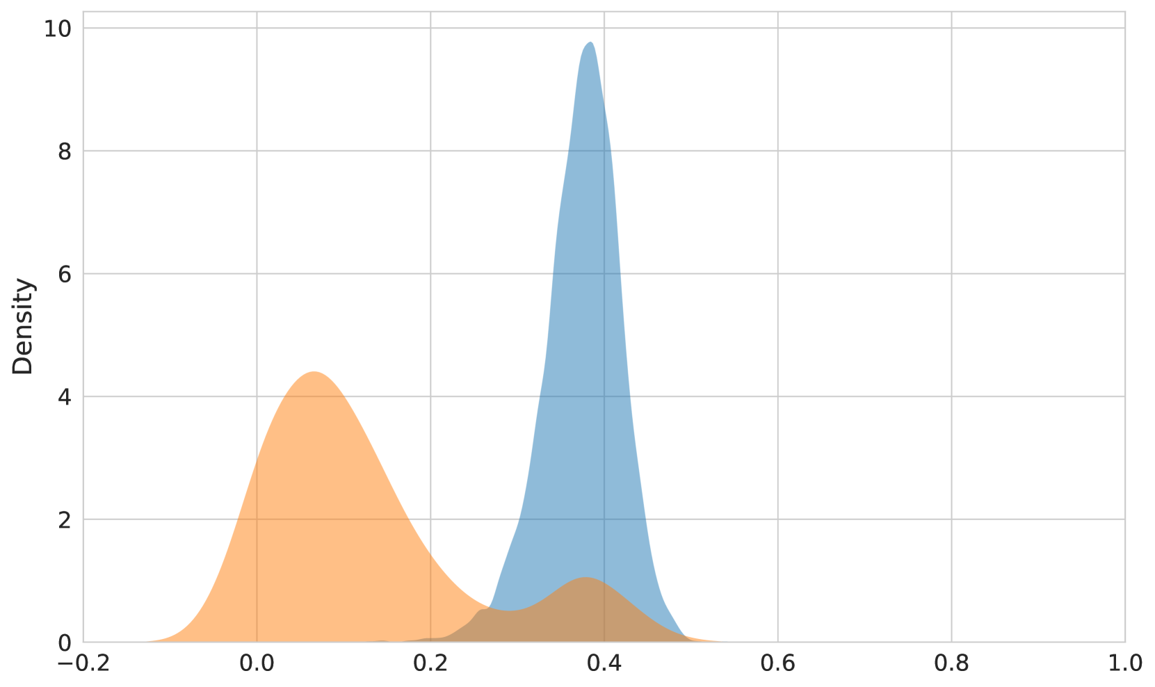
\n ## Density Plot: Bimodal Distribution ### Overview The image presents a density plot displaying a bimodal distribution. Two distinct peaks are visible, suggesting two underlying populations or clusters within the data. The x-axis ranges from -0.2 to 1.0, and the y-axis represents density, ranging from 0 to 10. ### Components/Axes * **X-axis:** Labeled "Density", ranging from -0.2 to 1.0. * **Y-axis:** Labeled "Density", ranging from 0 to 10. * **Data Series 1:** Filled curve in orange. * **Data Series 2:** Filled curve in blue. ### Detailed Analysis The plot shows two prominent peaks. * **Orange Curve:** This curve exhibits a peak around a density value of approximately 4, centered at approximately x = 0.05. The curve starts at x = -0.2, rises to the peak, and then declines towards x = 0.2. * **Blue Curve:** This curve has a more pronounced peak, reaching a density of approximately 9, centered around x = 0.35. The curve begins to rise around x = 0.2, reaches its peak at x = 0.35, and then gradually declines towards x = 0.7. The area under each curve represents the proportion of data belonging to that distribution. The blue curve has a larger area, indicating a greater proportion of data points are associated with that distribution. ### Key Observations * **Bimodality:** The most striking feature is the presence of two distinct peaks, indicating a bimodal distribution. * **Peak Heights:** The blue peak is significantly higher than the orange peak, suggesting a larger concentration of data points around x = 0.35. * **Distribution Spread:** The orange curve is wider than the blue curve, indicating a greater spread or variance in the data associated with that distribution. ### Interpretation The bimodal distribution suggests that the data originates from two different underlying processes or populations. The two peaks represent the most frequent values within each population. The difference in peak heights indicates that one population is more prevalent than the other. The data could represent a mixture of two different datasets, or a single dataset with two distinct subgroups. Further investigation would be needed to determine the cause of the bimodality and the characteristics of each population. For example, the data could represent the distribution of heights of men and women, or the distribution of test scores for two different teaching methods. The fact that the distributions are not perfectly separated suggests some overlap between the populations.