## Diagram: Expert Routing Mechanism with Temperature Scaling
### Overview
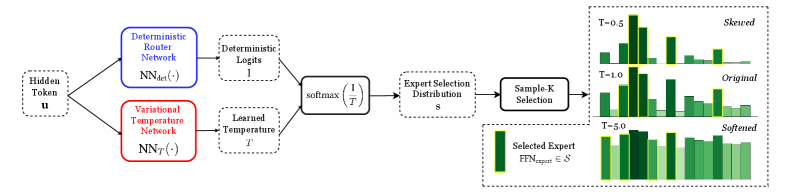
The image is a technical flowchart illustrating a machine learning model's routing mechanism. It depicts how an input "Hidden Token u" is processed through two parallel neural networks to produce a temperature-scaled distribution for selecting from a set of experts. The diagram emphasizes the effect of a learned temperature parameter on the final expert selection distribution, visualized through three comparative bar charts.
### Components/Axes
The diagram is structured as a left-to-right flowchart with the following labeled components and their spatial relationships:
1. **Input (Far Left):**
* `Hidden Token u`: The starting point of the process.
2. **Parallel Processing Branches (Left-Center):**
* **Top Branch (Blue Box):** `Deterministic Router Network` with the function notation `NN_det(·)`.
* **Bottom Branch (Red Box):** `Variational Temperature Network` with the function notation `NN_T(·)`.
3. **Intermediate Outputs (Center):**
* From the top branch: `Deterministic Logits l`.
* From the bottom branch: `Learned Temperature T`.
* These two outputs feed into a central processing block.
4. **Core Processing (Center):**
* A block labeled `softmax(1/T)`, indicating the application of a softmax function with an inverse temperature scaling factor.
* The output of this block is the `Expert Selection Distribution s`.
5. **Selection Mechanism (Center-Right):**
* A block labeled `Sample-K Selection`, which takes the distribution `s` as input.
6. **Output Visualization (Right Side):**
* Three bar charts are stacked vertically, each representing the expert selection distribution under a different temperature (`T`) value.
* **Top Chart:** Labeled `T=0.5` and `Skewed`.
* **Middle Chart:** Labeled `T=1.0` and `Original`.
* **Bottom Chart:** Labeled `T=5.0` and `Softened`.
* A legend at the bottom right indicates that the green bars represent the `Selected Expert f(x_input) ∈ S`.
### Detailed Analysis
The diagram details a specific computational flow:
1. A single input, the `Hidden Token u`, is fed simultaneously into two distinct neural networks.
2. The `Deterministic Router Network` produces a set of raw scores or `logits (l)`.
3. The `Variational Temperature Network` produces a scalar `temperature (T)`.
4. These two outputs are combined via a `softmax` function where the logits are scaled by `1/T`. This is a standard technique where:
* **T < 1 (e.g., T=0.5):** Amplifies differences between logits, leading to a sharper, more "skewed" distribution where one or a few experts have very high probability.
* **T = 1:** The "Original" or standard softmax distribution.
* **T > 1 (e.g., T=5.0):** Dampens differences between logits, leading to a "softened," more uniform distribution where probability is spread more evenly across experts.
5. The resulting `Expert Selection Distribution s` is then used by a `Sample-K Selection` mechanism to choose one or more experts.
6. The three bar charts on the right visually confirm the effect of temperature:
* **T=0.5 (Skewed):** One green bar (expert) is significantly taller than the others, indicating a high-confidence selection.
* **T=1.0 (Original):** The bar heights show a moderate variance, representing the baseline distribution.
* **T=5.0 (Softened):** All green bars are of nearly equal height, indicating a near-uniform, low-confidence selection across all experts.
### Key Observations
* **Dual-Network Architecture:** The system uses two separate networks to decouple the calculation of routing scores (logits) from the calculation of the routing confidence (temperature).
* **Temperature as a Control Parameter:** The learned temperature `T` acts as a dynamic, input-dependent knob that controls the entropy (or sharpness) of the expert selection policy.
* **Visual Trend Verification:** The bar charts clearly demonstrate the inverse relationship between temperature `T` and distribution sharpness. As `T` increases from 0.5 to 5.0, the distribution transitions from highly peaked (skewed) to nearly flat (softened).
* **Spatial Grounding:** The legend (`Selected Expert...`) is positioned in the bottom-right corner, directly below the three comparative charts it describes. The color green is consistently used for the bars representing selected experts across all three charts.
### Interpretation
This diagram illustrates a sophisticated **adaptive routing mechanism** for a mixture-of-experts (MoE) model. The core innovation is making the routing "temperature" a learnable function of the input itself, rather than a fixed hyperparameter.
* **What it suggests:** The model can dynamically decide, for each input token, whether to route it to a specific, specialized expert (low T, skewed distribution) or to distribute the computation more broadly across multiple generalist experts (high T, softened distribution). This allows for a balance between **specialization** (efficient, confident routing) and **exploration/robustness** (uncertain inputs get processed by multiple experts).
* **How elements relate:** The `Variational Temperature Network` is key. It analyzes the `Hidden Token u` and determines the appropriate level of routing confidence. This decision modulates the output of the `Deterministic Router Network` via the softmax scaling, directly influencing the final expert selection.
* **Notable implications:** This approach likely improves model performance and efficiency. For clear, in-distribution inputs, the model can commit to a single expert (saving compute). For ambiguous or novel inputs, it can hedge its bets by consulting multiple experts, potentially improving accuracy and robustness. The term "Variational" in the temperature network's name hints at a possible connection to variational inference, suggesting the temperature might be modeling an uncertainty parameter.