## 3D Scatter Plot Pair: Scaling Laws for Language Model Validation Loss
### Overview
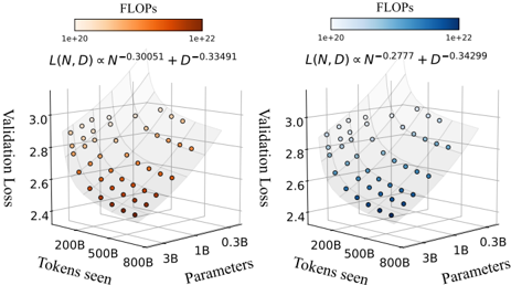
The image displays two side-by-side 3D scatter plots. Each plot visualizes the relationship between a language model's **Validation Loss** (vertical axis), the number of **Tokens seen** during training (left horizontal axis), and the model's size in **Parameters** (right horizontal axis). The color of each data point represents the computational cost in **FLOPs** (Floating Point Operations), following a logarithmic color scale. Each plot is annotated with a different empirical scaling law equation relating these variables.
### Components/Axes
**Common Elements (Both Plots):**
* **Chart Type:** 3D Scatter Plot
* **X-Axis (Left):** `Tokens seen`. Scale is logarithmic with major ticks at: `200B`, `500B`, `800B`, `1B`, `0.3B`. (Note: The order appears reversed, with larger values on the left).
* **Y-Axis (Right):** `Parameters`. Scale is logarithmic with major ticks at: `200B`, `500B`, `800B`, `1B`, `0.3B`. (Note: The order appears reversed, with larger values on the right).
* **Z-Axis (Vertical):** `Validation Loss`. Linear scale ranging from approximately `2.4` to `3.0`.
* **Color Bar (Top):** Labeled `FLOPs`. Logarithmic scale from `1e+20` (lightest) to `1e+22` (darkest).
* **Data Points:** Arranged in a 3D grid pattern, forming a surface.
**Left Plot Specifics:**
* **Color Gradient:** Warm tones (light orange to dark red/brown).
* **Scaling Law Equation (Top Center):** `L(N, D) ∝ N^0.30051 + D^0.33491`
* `L`: Validation Loss
* `N`: Parameters
* `D`: Tokens seen (Data)
**Right Plot Specifics:**
* **Color Gradient:** Cool tones (light blue to dark blue).
* **Scaling Law Equation (Top Center):** `L(N, D) ∝ N^0.2777 + D^0.34299`
### Detailed Analysis
**Data Point Distribution & Trends:**
1. **General Trend (Both Plots):** Validation Loss decreases as both the number of `Tokens seen` and the number of `Parameters` increase. The data points form a sloping surface, lowest (best loss) in the corner representing high tokens and high parameters, and highest (worst loss) in the opposite corner representing low tokens and low parameters.
2. **Color/FLOPs Trend:** In both plots, data points become darker (indicating higher FLOPs) as they move towards the high-parameter, high-token corner. This visually confirms that training larger models on more data requires exponentially more computation.
3. **Left Plot (Exponents ~0.30 & 0.33):** The surface appears slightly steeper along the `Parameters` axis compared to the right plot. This suggests the scaling law here gives a slightly higher weight to model size (`N`) in reducing loss.
4. **Right Plot (Exponents ~0.28 & 0.34):** The surface appears slightly steeper along the `Tokens seen` axis compared to the left plot. This suggests the scaling law here gives a slightly higher weight to data size (`D`) in reducing loss.
**Approximate Value Ranges:**
* **Validation Loss:** Ranges from a high of ~`3.0` (at low N, low D) to a low of ~`2.4` (at high N, high D).
* **FLOPs:** The color gradient spans two orders of magnitude, from `1e+20` to `1e+22`.
### Key Observations
1. **Diminishing Returns:** The surface flattens out as loss decreases, indicating diminishing returns. Adding more parameters or data yields smaller improvements in loss at the high end.
2. **Compute Color Correlation:** The perfect correlation between position (high N, high D) and dark color (high FLOPs) is a direct visual representation of the fundamental compute constraint in scaling laws: better performance requires more computation.
3. **Equation Sensitivity:** The two plots, with slightly different exponents, demonstrate how sensitive the predicted loss surface is to the precise values of the scaling coefficients. A small change in the exponent for `N` (0.30051 vs. 0.2777) visibly alters the shape of the loss landscape.
### Interpretation
These plots are a visual representation of **neural scaling laws**, which are empirical formulas predicting how a model's performance (here, validation loss) improves with increased scale (model size `N` and data size `D`) and compute (`FLOPs`).
* **What the Data Demonstrates:** The plots confirm the core hypothesis of scaling laws: loss follows a power-law relationship with both model and data size. The color gradient explicitly ties this performance gain to its cost in FLOPs.
* **Relationship Between Elements:** `Parameters` and `Tokens seen` are the independent variables we control. `Validation Loss` is the dependent outcome we measure. `FLOPs` is the consequential resource cost, roughly proportional to `N * D`. The two equations represent two different fits to experimental data, proposing slightly different balances between the importance of model size versus data size.
* **Notable Insight:** The comparison between the two plots highlights an active area of research: determining the optimal allocation of a fixed compute budget between making a model larger (`N`) versus training it on more data (`D`). The left plot's equation suggests a more balanced allocation, while the right plot's equation suggests a slightly stronger emphasis on data. The "best" law depends on the specific model architecture and training regime from which the data was derived. The uncertainty in the exponents (e.g., `0.30051`) underscores that these are empirical fits, not theoretical absolutes.