## Auditory Processing Diagram and Filter Response Charts
### Overview
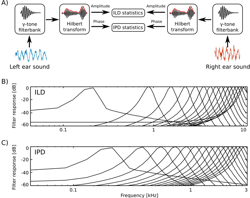
The image presents a diagram of auditory processing, followed by two charts illustrating filter responses for Interaural Level Difference (ILD) and Interaural Phase Difference (IPD). The diagram shows the processing of sound from the left and right ears, involving gamma-tone filterbanks, Hilbert transforms, and the extraction of ILD and IPD statistics. The charts display the filter response in decibels (dB) as a function of frequency in kilohertz (kHz).
### Components/Axes
**A) Auditory Processing Diagram:**
* **Left Side:**
* "Left ear sound": An example waveform in blue.
* "γ-tone filterbank": A block representing the filterbank, with an example waveform.
* "Hilbert transform": A block representing the Hilbert transform, with an example waveform and its envelope in red.
* "Amplitude": An arrow pointing from the Hilbert transform block to "ILD statistics".
* "Phase": An arrow pointing from the Hilbert transform block to "IPD statistics".
* **Right Side:**
* "Right ear sound": An example waveform in red.
* "γ-tone filterbank": A block representing the filterbank, with an example waveform.
* "Hilbert transform": A block representing the Hilbert transform, with an example waveform and its envelope in red.
* "Amplitude": An arrow pointing from the Hilbert transform block to "ILD statistics".
* "Phase": An arrow pointing from the Hilbert transform block to "IPD statistics".
* **Center:**
* "ILD statistics": A block representing the extraction of Interaural Level Difference statistics.
* "IPD statistics": A block representing the extraction of Interaural Phase Difference statistics.
**B) ILD Filter Response Chart:**
* **Y-axis:** "Filter response [dB]", ranging from -60 to 0 in increments of 20.
* **X-axis:** "Frequency [kHz]", ranging from 0.1 to 10 on a logarithmic scale.
* "ILD" label in the top-left corner of the chart.
* Multiple black lines representing different filter responses.
**C) IPD Filter Response Chart:**
* **Y-axis:** "Filter response [dB]", ranging from -60 to 0 in increments of 20.
* **X-axis:** "Frequency [kHz]", ranging from 0.1 to 3 on a logarithmic scale.
* "IPD" label in the top-left corner of the chart.
* Multiple black lines representing different filter responses.
### Detailed Analysis
**A) Auditory Processing Diagram:**
The diagram illustrates a binaural auditory processing model. Sound from each ear is processed through a gamma-tone filterbank, which decomposes the sound into different frequency channels. The Hilbert transform is then applied to each channel to extract the amplitude envelope and instantaneous phase. These amplitude and phase components are used to compute ILD and IPD statistics, which are crucial cues for sound localization.
**B) ILD Filter Response Chart:**
* The chart shows a set of filter responses.
* The lowest frequency filter peaks around 0.2 kHz with a response of approximately 0 dB.
* The filter responses generally increase in frequency, with the highest frequency filters peaking around 8-10 kHz.
* The filter responses are generally between -60 dB and 0 dB.
**C) IPD Filter Response Chart:**
* The chart shows a set of filter responses.
* The lowest frequency filter peaks around 0.2 kHz with a response of approximately 0 dB.
* The filter responses generally increase in frequency, with the highest frequency filters peaking around 2-3 kHz.
* The filter responses are generally between -60 dB and 0 dB.
### Key Observations
* The auditory processing diagram highlights the key steps in binaural hearing, from sound input to the extraction of spatial cues.
* The ILD and IPD filter response charts show the frequency selectivity of the auditory system for these spatial cues.
* The ILD filter responses extend to higher frequencies than the IPD filter responses, reflecting the fact that ILDs are more important for localizing high-frequency sounds.
### Interpretation
The image provides a concise overview of how the auditory system processes sound to extract spatial information. The diagram illustrates the flow of information from the ears to the computation of ILD and IPD statistics. The filter response charts demonstrate the frequency-dependent sensitivity of the auditory system to these spatial cues. This information is crucial for understanding how humans localize sounds in their environment. The model suggests that the brain analyzes both the amplitude and phase differences between the sounds arriving at each ear to determine the location of the sound source. The different frequency ranges for ILD and IPD sensitivity indicate that the auditory system uses different mechanisms for localizing sounds of different frequencies.