## Diagram: Auditory Localization Processing
### Overview
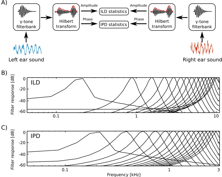
This image depicts a diagram illustrating the processing of auditory information for sound localization. It shows a signal processing pathway from left and right ear sound inputs to Interaural Level Difference (ILD) and Interaural Phase Difference (IPD) statistics, followed by two charts visualizing the filter responses for ILD and IPD across different frequencies.
### Components/Axes
The diagram consists of three main parts: A, B, and C.
* **Part A:** A flow diagram showing the processing steps. It includes components labeled: "Left ear sound", "γ-tone filterbank", "Hilbert transform", "Amplitude", "Phase", "ILD statistics", "IPD statistics", and "Right ear sound". Arrows indicate the direction of signal flow.
* **Part B:** A chart titled "ILD" (Interaural Level Difference). The x-axis is labeled "Frequency [kHz]" and ranges from approximately 0.01 to 10 kHz. The y-axis is labeled "Filter response [dB]" and ranges from 0 to -60 dB. Multiple lines represent filter responses at different levels.
* **Part C:** A chart titled "IPD" (Interaural Phase Difference). The x-axis is labeled "Frequency [kHz]" and ranges from approximately 0.01 to 3 kHz. The y-axis is labeled "Filter response [dB]" and ranges from 0 to -60 dB. Multiple lines represent filter responses at different levels.
### Detailed Analysis or Content Details
**Part A: Signal Processing Flow**
1. **Left ear sound:** An initial waveform representing sound input to the left ear.
2. **γ-tone filterbank:** The sound is processed by a γ-tone filterbank.
3. **Hilbert transform:** The output of the filterbank is then passed through a Hilbert transform, which separates the signal into Amplitude and Phase components.
4. **ILD statistics:** Amplitude information is used to calculate Interaural Level Difference (ILD) statistics.
5. **IPD statistics:** Phase information is used to calculate Interaural Phase Difference (IPD) statistics.
6. **Right ear sound:** An initial waveform representing sound input to the right ear.
7. **γ-tone filterbank:** The sound is processed by a γ-tone filterbank.
8. **Hilbert transform:** The output of the filterbank is then passed through a Hilbert transform, which separates the signal into Amplitude and Phase components.
**Part B: ILD Filter Responses**
The ILD chart displays multiple curves representing filter responses. The curves generally exhibit the following characteristics:
* **Low Frequencies (0.01 - ~0.5 kHz):** Most curves are relatively flat, near 0 dB.
* **Mid Frequencies (~0.5 - 2 kHz):** Curves begin to diverge, with some decreasing rapidly towards -60 dB.
* **High Frequencies (~2 - 10 kHz):** Curves continue to diverge, with a wider range of filter responses. Some curves remain near 0 dB, while others reach -60 dB.
* There are approximately 15 curves visible, each representing a different filter response. The curves are closely spaced, particularly at lower frequencies.
**Part C: IPD Filter Responses**
The IPD chart displays multiple curves representing filter responses. The curves generally exhibit the following characteristics:
* **Low Frequencies (0.01 - ~0.2 kHz):** Most curves are relatively flat, near 0 dB.
* **Mid Frequencies (~0.2 - 1 kHz):** Curves begin to diverge, with some decreasing rapidly towards -60 dB.
* **High Frequencies (~1 - 3 kHz):** Curves continue to diverge, with a wider range of filter responses. Some curves remain near 0 dB, while others reach -60 dB.
* There are approximately 15 curves visible, each representing a different filter response. The curves are closely spaced, particularly at lower frequencies.
### Key Observations
* The ILD chart shows a broader frequency range (up to 10 kHz) compared to the IPD chart (up to 3 kHz).
* Both ILD and IPD filter responses exhibit a frequency-dependent behavior, with greater differentiation at higher frequencies.
* The filter responses in both charts are diverse, suggesting a complex representation of auditory information.
* The curves in both charts are generally decreasing, indicating that the filter responses attenuate the signal at higher frequencies.
### Interpretation
This diagram illustrates how the auditory system processes sound to determine its location. The γ-tone filterbank decomposes the sound into different frequency components. The Hilbert transform extracts amplitude and phase information, which are then used to calculate ILD and IPD. These differences between the left and right ears provide cues for sound localization.
The ILD chart shows how the system filters different frequencies to extract level differences, which are particularly important for high-frequency sounds. The IPD chart shows how the system filters different frequencies to extract phase differences, which are particularly important for low-frequency sounds.
The diversity of filter responses suggests that the auditory system is capable of representing a wide range of sound localization cues. The frequency-dependent behavior of the filter responses indicates that the system prioritizes different cues at different frequencies. The attenuation of signals at higher frequencies may be related to the limitations of the auditory system or to the characteristics of natural sounds.