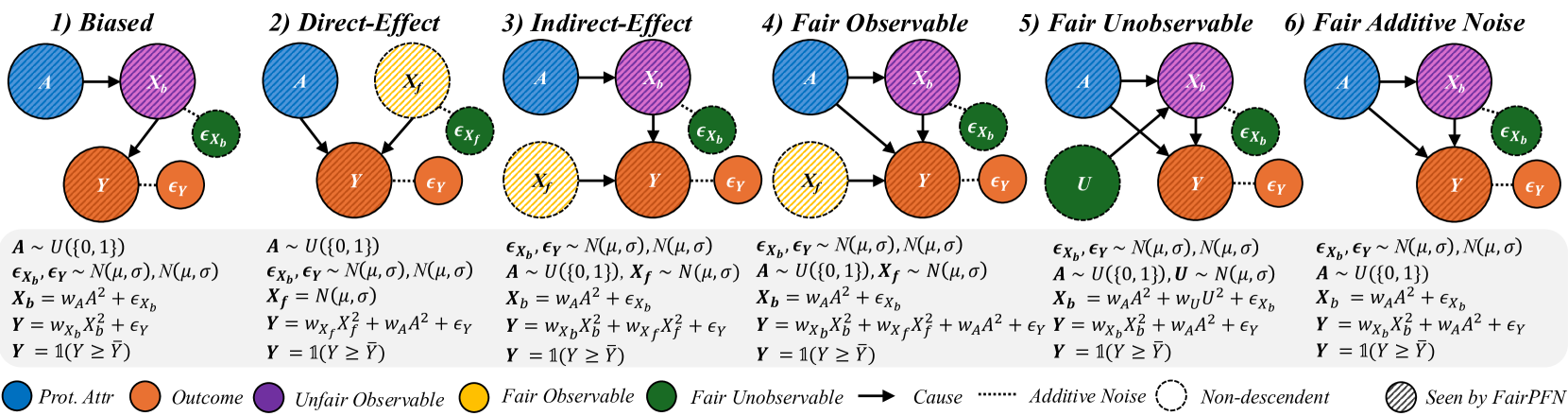
## Causal Diagram: Fairness Scenarios ### Overview The image presents six causal diagrams illustrating different scenarios related to fairness and bias in machine learning models. Each diagram depicts relationships between protected attributes, outcomes, and other variables, highlighting potential sources of unfairness. ### Components/Axes * **Nodes:** Represent variables. * Blue, diagonally-striped circle: Prot. Attr (Protected Attribute) * Orange, diagonally-striped circle: Outcome * Yellow, dashed-outline circle: Fair Observable * Purple, diagonally-striped circle: Unfair Observable * Green, dashed-outline circle: Fair Unobservable * **Edges:** Represent causal relationships. * Solid arrow: Cause * Dotted line: Additive Noise * Dashed line: Non-descendent * **Text:** * Titles above each diagram: 1) Biased, 2) Direct-Effect, 3) Indirect-Effect, 4) Fair Observable, 5) Fair Unobservable, 6) Fair Additive Noise * Equations and distributions below the diagrams defining the relationships between variables. * **Legend:** Located at the bottom of the image, explaining the meaning of the node colors and edge types. * "Prot. Attr": Blue, diagonally-striped circle * "Outcome": Orange, diagonally-striped circle * "Unfair Observable": Purple, diagonally-striped circle * "Fair Observable": Yellow, dashed-outline circle * "Fair Unobservable": Green, dashed-outline circle * "Cause": Solid arrow * "Additive Noise": Dotted line * "Non-descendent": Dashed line * "Seen by FairPFN": Diagonally-striped fill ### Detailed Analysis or Content Details Each diagram includes the following variables: * A: Protected Attribute (blue, diagonally-striped) * Y: Outcome (orange, diagonally-striped) * Xb: Unfair Observable (purple, diagonally-striped) * Xf: Fair Observable (yellow, dashed-outline) * U: Fair Unobservable (green, dashed-outline) * εXb, εXf, εY: Additive Noise (green, dashed-outline or orange, dashed-outline) **1) Biased:** * A -> Xb -> Y * Y has additive noise εY * Xb has additive noise εXb * Equations: * A ~ U({0, 1}) * εXb, εY ~ N(μ, σ), N(μ, σ) * Xb = wAA² + εXb * Y = wXbXb² + εY * Y = 1(Y ≥ Ȳ) **2) Direct-Effect:** * A -> Y * Xf -> Y * Y has additive noise εY * Xf has additive noise εXf * Equations: * A ~ U({0, 1}) * εXf, εY ~ N(μ, σ), N(μ, σ) * Xf = N(μ, σ) * Y = wXfXf² + wAA² + εY * Y = 1(Y ≥ Ȳ) **3) Indirect-Effect:** * A -> Xb -> Y * Xf -> Y * Y has additive noise εY * Xb has additive noise εXb * Equations: * εXb, εY ~ N(μ, σ), N(μ, σ) * A ~ U({0, 1}), Xf ~ N(μ, σ) * Xb = wAA² + εXb * Y = wXbXb² + wXfXf² + εY * Y = 1(Y ≥ Ȳ) **4) Fair Observable:** * A -> Xb -> Y * A -> Xf -> Y * Y has additive noise εY * Xb has additive noise εXb * Equations: * εXb, εY ~ N(μ, σ), N(μ, σ) * A ~ U({0, 1}), Xf ~ N(μ, σ) * Xb = wAA² + εXb * Y = wXbXb² + wXfXf² + wAA² + εY * Y = 1(Y ≥ Ȳ) **5) Fair Unobservable:** * A -> Xb -> Y * U -> Xb -> Y * A -> Y * U -> Y * Y has additive noise εY * Xb has additive noise εXb * Equations: * εXb, εY ~ N(μ, σ), N(μ, σ) * A ~ U({0, 1}), U ~ N(μ, σ) * Xb = wAA² + wUU² + εXb * Y = wXbXb² + wAA² + εY * Y = 1(Y ≥ Ȳ) **6) Fair Additive Noise:** * A -> Xb -> Y * Y has additive noise εY * Xb has additive noise εXb * Equations: * εXb, εY ~ N(μ, σ), N(μ, σ) * A ~ U({0, 1}) * Xb = wAA² + εXb * Y = wXbXb² + wAA² + εY * Y = 1(Y ≥ Ȳ) ### Key Observations * The diagrams illustrate different ways in which a protected attribute (A) can influence an outcome (Y), either directly or indirectly through other variables. * The presence of "fair" and "unfair" observables (Xf and Xb) highlights the potential for bias to be introduced or mitigated depending on which variables are used in a model. * Additive noise (ε) is present in all diagrams, representing random variation or unobserved factors. * The equations below each diagram provide a mathematical representation of the relationships between the variables. * The thresholding function Y = 1(Y ≥ Ȳ) suggests a classification task where the outcome is binary. ### Interpretation The diagrams demonstrate how different causal structures can lead to biased outcomes. Understanding these structures is crucial for developing fair machine learning models. The diagrams highlight the importance of considering the relationships between protected attributes, outcomes, and other variables, as well as the potential for bias to be introduced through various pathways. The scenarios presented provide a framework for analyzing and mitigating bias in real-world applications. The use of both observable and unobservable variables emphasizes the challenges of achieving fairness when not all relevant information is available.

\n ## Diagram: Fairness Scenarios in Machine Learning ### Overview The image presents a series of six diagrams illustrating different scenarios related to fairness in machine learning models. Each scenario depicts a causal diagram with nodes representing protected attributes, unfair observable features, fair observable features, outcomes, and error terms. The diagrams aim to visualize how different types of bias and unfairness can manifest in a model's decision-making process. ### Components/Axes The diagrams share the following components: * **Protected Attribute (Prot. Attr):** Represented by a teal-colored circle labeled "A". * **Outcome:** Represented by a purple circle labeled "Y". * **Unfair Observable:** Represented by an orange circle labeled "X_b". * **Fair Observable:** Represented by a yellow circle labeled "X_f". * **Error Terms:** Represented by small, light-blue circles labeled "ε_x" and "ε_y". * **Arrows:** Indicate causal relationships between variables. * **Legend:** Located at the bottom-right, defining the color-coding for each component. * **Mathematical Equations:** Below each diagram, defining the relationships between variables. * **Titles:** Above each diagram, indicating the fairness scenario (1) Biased, (2) Direct-Effect, (3) Indirect-Effect, (4) Fair Observable, (5) Fair Unobservable, (6) Fair Additive Noise. ### Content Details Here's a breakdown of each scenario, including the equations: **1) Biased:** * A -> X_b -> Y * A -> X_f -> Y * Equation: A ~ U(0,1), ε_x, ε_y ~ N(μ,0), σ, X_b = W_A² + ε_x, X_f = W_A² + ε_x, Y = W_xX_b + W_xX_f + ε_y, Y = 1(Y ≥ γ) **2) Direct-Effect:** * A -> X_b -> Y * A -> X_f * Equation: A ~ U(0,1), X_b ~ N(μ_A,0), X_f ~ N(μ₀,0), X_f = N(μ₀), Y = W_xX_b + W_xX_f + ε_y, Y = 1(Y ≥ γ) **3) Indirect-Effect:** * A -> X_f -> X_b -> Y * Equation: ε_x, ε_y ~ N(μ,0), A ~ U(0,1), X_f ~ N(μ₀), X_b = W_A² + ε_x, Y = W_xX_b + W_xX_f + ε_y, Y = 1(Y ≥ γ) **4) Fair Observable:** * A -> X_f -> Y * Equation: ε_x, ε_y ~ N(μ,0), A ~ U(0,1), X_f ~ N(μ₀), X_b = W_A² + ε_x, Y = W_xX_b + W_xX_f + ε_y, Y = 1(Y ≥ γ) **5) Fair Unobservable:** * A -> U -> X_b -> Y * Equation: ε_x, ε_y ~ N(μ,0), A ~ U(0,1), U ~ N(μ₀), X_b = W_A² + W_U¹ + ε_x, Y = W_xX_b + W_xX_f + ε_y, Y = 1(Y ≥ γ) **6) Fair Additive Noise:** * A -> X_b -> Y * Equation: ε_x, ε_y ~ N(μ,0), A ~ U(0,1), X_b = W_A² + ε_x, X_f = W_A² + ε_x, Y = W_xX_b + W_xX_f + ε_y, Y = 1(Y ≥ γ) ### Key Observations * The diagrams consistently use the same node representations and causal arrow style. * The mathematical equations provide a formal definition of the relationships depicted in each diagram. * The scenarios vary in how the protected attribute (A) influences the outcome (Y), either directly, indirectly, or through observable/unobservable features. * The inclusion of error terms (ε_x, ε_y) acknowledges the inherent noise and uncertainty in real-world data. * The use of U(0,1) indicates a uniform distribution, while N(μ,σ) indicates a normal distribution. ### Interpretation These diagrams illustrate different ways in which bias can enter a machine learning model and affect its fairness. They highlight the importance of considering causal relationships when evaluating and mitigating bias. * **Scenario 1 (Biased):** Demonstrates a simple case where the protected attribute directly influences both observable features and the outcome, leading to potential discrimination. * **Scenario 2 (Direct-Effect):** Shows a direct causal link between the protected attribute and the outcome, bypassing observable features. * **Scenario 3 (Indirect-Effect):** Illustrates how the protected attribute can indirectly influence the outcome through a fair observable feature. * **Scenario 4 (Fair Observable):** Suggests a scenario where fairness is achieved by ensuring that the observable features are independent of the protected attribute. * **Scenario 5 (Fair Unobservable):** Introduces an unobservable variable (U) that mediates the relationship between the protected attribute and the outcome. * **Scenario 6 (Fair Additive Noise):** Represents a scenario where fairness is achieved by adding noise to the model's predictions. The diagrams, combined with the mathematical equations, provide a rigorous framework for analyzing and addressing fairness concerns in machine learning. They emphasize the need to understand the underlying causal mechanisms that drive bias and to develop interventions that target those mechanisms effectively. The "Seen by FairPFN" label at the bottom right suggests these diagrams are related to a specific fairness-aware machine learning framework or algorithm.

## Causal Diagram: Six Fairness Models in Machine Learning ### Overview The image displays six distinct causal models, numbered 1 through 6, illustrating different relationships between a protected attribute (`A`), observable features (`X_b`, `X_f`), an unobservable feature (`U`), an outcome (`Y`), and additive noise terms (`ε`). Each model is presented as a panel containing a directed acyclic graph (DAG) and its corresponding mathematical formulation. A legend at the bottom defines the visual symbols and node colors. ### Components/Axes The image is organized into six horizontal panels. Each panel contains: 1. **Title**: A numbered label (e.g., "1) Biased"). 2. **Causal Graph**: A diagram with colored nodes and arrows. 3. **Mathematical Formulation**: A set of equations defining the distributions and relationships between variables. **Legend (Bottom of Image):** * **Node Colors & Meanings**: * Blue Circle: `Prot. Attr.` (Protected Attribute, `A`) * Orange Circle: `Outcome` (`Y`) * Purple Circle: `Unfair Observable` (`X_b`) * Yellow Circle: `Fair Observable` (`X_f`) * Green Circle: `Fair Unobservable` (`U`) * **Arrow Types**: * Solid Arrow (`→`): `Cause` * Dotted Arrow (`⋯>`): `Additive Noise` * **Node Border**: * Dashed Circle Border: `Non-descendent` * **Node Fill Pattern**: * Hatched Pattern: `Seen by FairPFN` ### Detailed Analysis #### Panel 1: Biased * **Graph**: `A` (blue, hatched) → `X_b` (purple, hatched) → `Y` (orange, hatched). `X_b` has an additive noise term `ε_Xb` (green). `Y` has an additive noise term `ε_Y` (orange). * **Equations**: * `A ~ U({0,1})` * `ε_Xb, ε_Y ~ N(μ, σ), N(μ, σ)` * `X_b = w_A * A² + ε_Xb` * `Y = w_Xb * X_b² + ε_Y` * `Y = 1(Y ≥ Ȳ)` #### Panel 2: Direct-Effect * **Graph**: `A` (blue, hatched) → `X_f` (yellow, hatched) → `Y` (orange, hatched). `A` also has a direct arrow to `Y`. `X_f` has an additive noise term `ε_Xf` (green). `Y` has an additive noise term `ε_Y` (orange). * **Equations**: * `A ~ U({0,1})` * `ε_Xb, ε_Y ~ N(μ, σ), N(μ, σ)` * `X_f = N(μ, σ)` * `Y = w_Xf * X_f² + w_A * A² + ε_Y` * `Y = 1(Y ≥ Ȳ)` #### Panel 3: Indirect-Effect * **Graph**: `A` (blue, hatched) → `X_b` (purple, hatched) → `Y` (orange, hatched). `X_f` (yellow, dashed border) → `Y`. `X_b` has an additive noise term `ε_Xb` (green). `Y` has an additive noise term `ε_Y` (orange). * **Equations**: * `ε_Xb, ε_Y ~ N(μ, σ), N(μ, σ)` * `A ~ U({0,1}), X_f ~ N(μ, σ)` * `X_b = w_A * A² + ε_Xb` * `Y = w_Xb * X_b² + w_Xf * X_f² + ε_Y` * `Y = 1(Y ≥ Ȳ)` #### Panel 4: Fair Observable * **Graph**: `A` (blue, hatched) → `X_b` (purple, hatched) → `Y` (orange, hatched). `A` also has a direct arrow to `Y`. `X_f` (yellow, dashed border) → `Y`. `X_b` has an additive noise term `ε_Xb` (green). `Y` has an additive noise term `ε_Y` (orange). * **Equations**: * `ε_Xb, ε_Y ~ N(μ, σ), N(μ, σ)` * `A ~ U({0,1}), X_f ~ N(μ, σ)` * `X_b = w_A * A² + ε_Xb` * `Y = w_Xb * X_b² + w_Xf * X_f² + w_A * A² + ε_Y` * `Y = 1(Y ≥ Ȳ)` #### Panel 5: Fair Unobservable * **Graph**: `A` (blue, hatched) → `X_b` (purple, hatched) → `Y` (orange, hatched). `A` also has a direct arrow to `Y`. `U` (green, dashed border) → `X_b` and `U` → `Y`. `X_b` has an additive noise term `ε_Xb` (green). `Y` has an additive noise term `ε_Y` (orange). * **Equations**: * `ε_Xb, ε_Y ~ N(μ, σ), N(μ, σ)` * `A ~ U({0,1}), U ~ N(μ, σ)` * `X_b = w_A * A² + w_U * U² + ε_Xb` * `Y = w_Xb * X_b² + w_A * A² + ε_Y` * `Y = 1(Y ≥ Ȳ)` #### Panel 6: Fair Additive Noise * **Graph**: `A` (blue, hatched) → `X_b` (purple, hatched) → `Y` (orange, hatched). `A` also has a direct arrow to `Y`. `X_b` has an additive noise term `ε_Xb` (green). `Y` has an additive noise term `ε_Y` (orange). * **Equations**: * `ε_Xb, ε_Y ~ N(μ, σ), N(μ, σ)` * `A ~ U({0,1})` * `X_b = w_A * A² + ε_Xb` * `Y = w_Xb * X_b² + w_A * A² + ε_Y` * `Y = 1(Y ≥ Ȳ)` ### Key Observations 1. **Progression of Complexity**: The models progress from a simple biased pathway (1) to more complex structures incorporating direct effects (2, 4, 6), indirect effects (3), and unobservable confounders (5). 2. **Variable Roles**: The protected attribute `A` is always binary (`U({0,1})`). The outcome `Y` is always binarized via a threshold (`1(Y ≥ Ȳ)`). Observable features (`X_b`, `X_f`) and the unobservable `U` are modeled with normal distributions. 3. **Visual Coding**: The hatched pattern indicates which variables are "Seen by FairPFN," suggesting this diagram is from a paper proposing or analyzing a method called FairPFN. The dashed border for `X_f` and `U` in panels 3, 4, and 5 marks them as "Non-descendent" of `A` in those specific causal structures. 4. **Mathematical Consistency**: All models use squared terms (e.g., `A²`, `X_b²`) in their structural equations, implying non-linear relationships. The noise terms are consistently modeled as Gaussian. ### Interpretation This diagram is a technical taxonomy of data-generating processes used to study algorithmic fairness. It systematically varies the causal pathways through which a protected attribute (`A`) can influence an outcome (`Y`). * **Model 1 (Biased)** represents a scenario where bias flows entirely through a single, unfair observable feature (`X_b`). * **Models 2 & 6 (Direct-Effect, Fair Additive Noise)** introduce a direct effect of `A` on `Y`, which is often considered a source of unfair discrimination. * **Model 3 (Indirect-Effect)** separates features into fair (`X_f`) and unfair (`X_b`) observables, with `A` only affecting `Y` through the unfair one. * **Model 4 (Fair Observable)** combines direct effect with both fair and unfair observable pathways. * **Model 5 (Fair Unobservable)** is the most complex, introducing an unobserved confounder (`U`) that affects both the unfair feature and the outcome, representing real-world complexity where important factors are not measured. The core purpose is to provide a framework for evaluating fairness interventions (like the mentioned "FairPFN"). By defining these precise data-generating models, researchers can test whether a fairness algorithm works correctly under different, well-specified assumptions about how bias enters a system. The consistent use of squared terms and Gaussian noise creates a controlled, synthetic environment for this evaluation. The diagram argues that understanding fairness requires moving beyond simple correlations to explicitly model the causal structure of the data.

## Causal Diagram: Fairness in Machine Learning Models ### Overview The image presents six causal diagrams illustrating different fairness scenarios in machine learning models. Each panel represents a distinct causal structure with variables, equations, and fairness constraints. The diagrams use color-coded nodes and arrows to depict relationships between protected attributes (A), outcomes (Y), and confounding variables (X_b, X_f). Equations quantify these relationships, while a legend at the bottom explains color/symbol meanings. ### Components/Axes - **Panels**: Six labeled scenarios (1-6) with distinct causal structures. - **Nodes**: - **Blue**: Protected Attribute (A) - **Purple**: Unfair Observable (X_b) - **Yellow**: Fair Observable (X_f) - **Green**: Fair Unobservable (U) - **Orange**: Outcome (Y) - **Arrows**: Indicate causal relationships (solid = direct cause, dashed = additive noise). - **Equations**: Mathematical formulations of relationships under each panel. - **Legend**: Located at the bottom, mapping colors/symbols to concepts (e.g., "Fair Observable," "Additive Noise"). ### Detailed Analysis #### Panel 1: Biased - **Structure**: A → X_b → Y with noise terms (ε_Xb, ε_Y). - **Equations**: - X_b = w_A*A² + ε_Xb - Y = w_Xb*X_b² + ε_Y - Y = 1(Y ≥ Ÿ) - **Key Features**: Direct bias from A to Y via X_b. #### Panel 2: Direct-Effect - **Structure**: A → X_f → Y with X_b as a confounder. - **Equations**: - X_f ~ N(μ,σ) - X_b = w_A*A² + ε_Xb - Y = w_Xf*X_f² + w_A*A² + ε_Y - **Key Features**: Introduces fair observable X_f to mitigate bias. #### Panel 3: Indirect-Effect - **Structure**: A → X_b → Y and A → X_f → Y. - **Equations**: - X_b = w_A*A² + ε_Xb - X_f ~ N(μ,σ) - Y = w_Xb*X_b² + w_Xf*X_f² + ε_Y - **Key Features**: Combines direct and indirect effects of A. #### Panel 4: Fair Observable - **Structure**: A → X_b → Y with X_f as a fair observable. - **Equations**: - X_b = w_A*A² + ε_Xb - X_f ~ N(μ,σ) - Y = w_Xb*X_b² + w_Xf*X_f² + w_A*A² + ε_Y - **Key Features**: Explicitly models fair observables to address bias. #### Panel 5: Fair Unobservable - **Structure**: A → X_b → Y with unobservable U. - **Equations**: - U ~ N(μ,σ) - X_b = w_A*A² + ε_Xb - Y = w_Xb*X_b² + w_A*U² + ε_Y - **Key Features**: Accounts for unobservable confounders (U). #### Panel 6: Fair Additive Noise - **Structure**: A → X_b → Y with additive noise. - **Equations**: - X_b = w_A*A² + ε_Xb - Y = w_Xb*X_b² + w_A*A² + ε_Y - **Key Features**: Adds noise to balance fairness constraints. ### Key Observations 1. **Color Consistency**: All panels use the same color scheme (blue for A, orange for Y, etc.), ensuring cross-panel comparability. 2. **Noise Terms**: ε_Xb and ε_Y appear in all panels, representing inherent variability. 3. **Fairness Mechanisms**: - Panels 2-6 introduce fairness constraints (e.g., X_f, U, additive noise) to counteract bias. - Panels 4-6 explicitly model fairness observables/unobservables. 4. **Equation Complexity**: Later panels (4-6) include more terms, reflecting advanced fairness adjustments. ### Interpretation The diagrams illustrate progressive strategies to address bias in causal models: - **Panel 1** represents a naive, biased model where A directly influences Y through X_b. - **Panels 2-3** introduce fairness observables (X_f) to disentangle direct/indirect effects. - **Panels 4-5** address observability challenges by incorporating fair unobservables (U) or adjusting for confounders. - **Panel 6** uses additive noise to balance fairness, ensuring Y is not disproportionately influenced by A. The equations reveal that fairness interventions often involve adding terms (e.g., w_A*A²) or noise to neutralize bias. The use of "FairPFN" (Fair Probabilistic Fairness Notion) in the legend suggests a framework for evaluating these models. Notably, all panels condition Y on a threshold (Y ≥ Ÿ), implying a focus on binary outcomes or fairness thresholds.