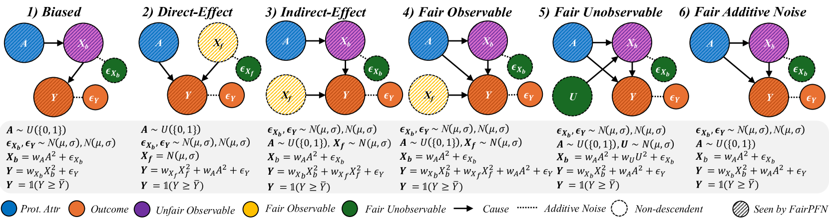
## Causal Diagram: Fairness in Machine Learning Models ### Overview The image presents six causal diagrams illustrating different fairness scenarios in machine learning models. Each panel represents a distinct causal structure with variables, equations, and fairness constraints. The diagrams use color-coded nodes and arrows to depict relationships between protected attributes (A), outcomes (Y), and confounding variables (X_b, X_f). Equations quantify these relationships, while a legend at the bottom explains color/symbol meanings. ### Components/Axes - **Panels**: Six labeled scenarios (1-6) with distinct causal structures. - **Nodes**: - **Blue**: Protected Attribute (A) - **Purple**: Unfair Observable (X_b) - **Yellow**: Fair Observable (X_f) - **Green**: Fair Unobservable (U) - **Orange**: Outcome (Y) - **Arrows**: Indicate causal relationships (solid = direct cause, dashed = additive noise). - **Equations**: Mathematical formulations of relationships under each panel. - **Legend**: Located at the bottom, mapping colors/symbols to concepts (e.g., "Fair Observable," "Additive Noise"). ### Detailed Analysis #### Panel 1: Biased - **Structure**: A → X_b → Y with noise terms (ε_Xb, ε_Y). - **Equations**: - X_b = w_A*A² + ε_Xb - Y = w_Xb*X_b² + ε_Y - Y = 1(Y ≥ Ÿ) - **Key Features**: Direct bias from A to Y via X_b. #### Panel 2: Direct-Effect - **Structure**: A → X_f → Y with X_b as a confounder. - **Equations**: - X_f ~ N(μ,σ) - X_b = w_A*A² + ε_Xb - Y = w_Xf*X_f² + w_A*A² + ε_Y - **Key Features**: Introduces fair observable X_f to mitigate bias. #### Panel 3: Indirect-Effect - **Structure**: A → X_b → Y and A → X_f → Y. - **Equations**: - X_b = w_A*A² + ε_Xb - X_f ~ N(μ,σ) - Y = w_Xb*X_b² + w_Xf*X_f² + ε_Y - **Key Features**: Combines direct and indirect effects of A. #### Panel 4: Fair Observable - **Structure**: A → X_b → Y with X_f as a fair observable. - **Equations**: - X_b = w_A*A² + ε_Xb - X_f ~ N(μ,σ) - Y = w_Xb*X_b² + w_Xf*X_f² + w_A*A² + ε_Y - **Key Features**: Explicitly models fair observables to address bias. #### Panel 5: Fair Unobservable - **Structure**: A → X_b → Y with unobservable U. - **Equations**: - U ~ N(μ,σ) - X_b = w_A*A² + ε_Xb - Y = w_Xb*X_b² + w_A*U² + ε_Y - **Key Features**: Accounts for unobservable confounders (U). #### Panel 6: Fair Additive Noise - **Structure**: A → X_b → Y with additive noise. - **Equations**: - X_b = w_A*A² + ε_Xb - Y = w_Xb*X_b² + w_A*A² + ε_Y - **Key Features**: Adds noise to balance fairness constraints. ### Key Observations 1. **Color Consistency**: All panels use the same color scheme (blue for A, orange for Y, etc.), ensuring cross-panel comparability. 2. **Noise Terms**: ε_Xb and ε_Y appear in all panels, representing inherent variability. 3. **Fairness Mechanisms**: - Panels 2-6 introduce fairness constraints (e.g., X_f, U, additive noise) to counteract bias. - Panels 4-6 explicitly model fairness observables/unobservables. 4. **Equation Complexity**: Later panels (4-6) include more terms, reflecting advanced fairness adjustments. ### Interpretation The diagrams illustrate progressive strategies to address bias in causal models: - **Panel 1** represents a naive, biased model where A directly influences Y through X_b. - **Panels 2-3** introduce fairness observables (X_f) to disentangle direct/indirect effects. - **Panels 4-5** address observability challenges by incorporating fair unobservables (U) or adjusting for confounders. - **Panel 6** uses additive noise to balance fairness, ensuring Y is not disproportionately influenced by A. The equations reveal that fairness interventions often involve adding terms (e.g., w_A*A²) or noise to neutralize bias. The use of "FairPFN" (Fair Probabilistic Fairness Notion) in the legend suggests a framework for evaluating these models. Notably, all panels condition Y on a threshold (Y ≥ Ÿ), implying a focus on binary outcomes or fairness thresholds.