## Line Graph: Shannon and Bayesian Surprises
### Overview
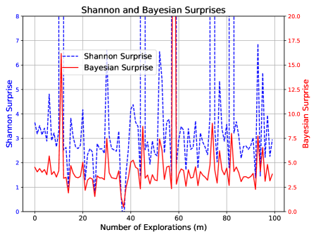
The image is a line graph comparing two metrics—**Shannon Surprise** (blue dashed line) and **Bayesian Surprise** (red solid line)—across a range of "Number of Explorations (m)" from 0 to 100. The graph includes dual y-axes: the left axis measures Shannon Surprise (0–8), and the right axis measures Bayesian Surprise (0–20). Both lines exhibit periodic spikes, but with distinct patterns and magnitudes.
---
### Components/Axes
- **Title**: "Shannon and Bayesian Surprises" (centered at the top).
- **Legend**: Located in the top-left corner, with:
- **Blue dashed line**: Labeled "Shannon Surprise."
- **Red solid line**: Labeled "Bayesian Surprise."
- **X-axis**:
- Label: "Number of Explorations (m)."
- Scale: 0 to 100, with markers at 0, 20, 40, 60, 80, 100.
- **Y-axes**:
- **Left (Shannon Surprise)**: 0 to 8, with increments of 1.
- **Right (Bayesian Surprise)**: 0 to 20, with increments of 2.5.
---
### Detailed Analysis
1. **Shannon Surprise (Blue Dashed Line)**:
- **Trend**: Exhibits frequent, smaller spikes at regular intervals (~20m, 40m, 60m, 80m, 100m).
- **Peak Values**: Approximately 6–7 at 20m, 40m, and 100m; lower (~3–4) at 60m and 80m.
- **Baseline**: Fluctuates between 1–3 between spikes.
2. **Bayesian Surprise (Red Solid Line)**:
- **Trend**: Fewer, larger spikes, primarily at 60m and 100m.
- **Peak Values**: Reaches ~17.5 at 60m and ~15 at 100m.
- **Baseline**: Remains near 0–2.5 except during spikes.
3. **Divergence**:
- The two lines rarely overlap. Bayesian Surprise peaks later (60m and 100m) compared to Shannon Surprise (20m, 40m, etc.).
- Bayesian Surprise magnitudes are consistently higher (up to 20 vs. 8 for Shannon).
---
### Key Observations
- **Periodicity**: Both metrics show periodic behavior, but Shannon Surprise is more regular (~20m intervals), while Bayesian Surprise is irregular.
- **Magnitude**: Bayesian Surprise values are ~2–3x higher than Shannon Surprise at their peaks.
- **Anomalies**:
- At 60m, Bayesian Surprise spikes sharply (~17.5), while Shannon Surprise remains low (~2).
- At 100m, both lines peak, but Bayesian Surprise (~15) dominates.
---
### Interpretation
The graph suggests that **Shannon Surprise** and **Bayesian Surprise** measure different aspects of uncertainty or information gain during explorations:
- **Shannon Surprise** (blue) reflects frequent, smaller surprises, possibly tied to immediate or local changes in the system. Its regularity implies a stable, predictable pattern of uncertainty.
- **Bayesian Surprise** (red) captures larger, less frequent surprises, potentially linked to global or model-specific updates. Its delayed peaks (60m and 100m) suggest it integrates information over longer exploration periods.
The divergence in peak positions and magnitudes indicates that the two metrics respond differently to the number of explorations. Bayesian Surprise may prioritize cumulative evidence, while Shannon Surprise reacts to discrete events. This could inform decisions in fields like machine learning, where balancing local and global uncertainty is critical.