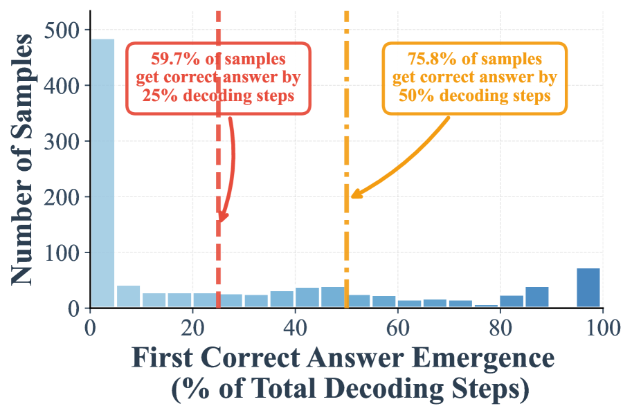
## Histogram: First Correct Answer Emergence in Decoding Steps
### Overview
This image is a histogram chart illustrating the distribution of when a model first produces a correct answer during a decoding process, measured as a percentage of the total decoding steps allocated. The chart includes two key annotations highlighting cumulative percentages at specific thresholds.
### Components/Axes
* **Chart Type:** Histogram (bar chart).
* **X-Axis:** Labeled **"First Correct Answer Emergence (% of Total Decoding Steps)"**. The scale runs from 0 to 100 in increments of 20 (0, 20, 40, 60, 80, 100). The axis represents the point in the decoding process (as a percentage of total steps) where the correct answer first appears.
* **Y-Axis:** Labeled **"Number of Samples"**. The scale runs from 0 to 500 in increments of 100 (0, 100, 200, 300, 400, 500). This represents the count of test samples (e.g., prompts or problems) for which the first correct answer emerged at the corresponding x-axis percentage.
* **Data Series:** A single series represented by light blue bars. The bar at the far right (95-100%) is a darker shade of blue.
* **Annotations:**
1. **Red Annotation (Top-Left):** A red-bordered text box stating **"59.7% of samples get correct answer by 25% decoding steps"**. A red dashed vertical line extends from this box down to the x-axis at the 25% mark. A red arrow points from the text box to this line.
2. **Orange Annotation (Top-Right):** An orange-bordered text box stating **"75.8% of samples get correct answer by 50% decoding steps"**. An orange dashed vertical line extends from this box down to the x-axis at the 50% mark. An orange arrow points from the text box to this line.
### Detailed Analysis
The histogram displays the frequency distribution across bins representing 5% intervals of the decoding process (e.g., 0-5%, 5-10%, ..., 95-100%).
* **Bar Values (Approximate):**
* **0-5%:** ~485 samples (The tallest bar by a significant margin).
* **5-10%:** ~40 samples.
* **10-15%:** ~25 samples.
* **15-20%:** ~25 samples.
* **20-25%:** ~25 samples.
* **25-30%:** ~25 samples.
* **30-35%:** ~25 samples.
* **35-40%:** ~30 samples.
* **40-45%:** ~35 samples.
* **45-50%:** ~40 samples.
* **50-55%:** ~25 samples.
* **55-60%:** ~20 samples.
* **60-65%:** ~15 samples.
* **65-70%:** ~15 samples.
* **70-75%:** ~10 samples.
* **75-80%:** ~5 samples.
* **80-85%:** ~20 samples.
* **85-90%:** ~40 samples.
* **90-95%:** ~10 samples.
* **95-100%:** ~75 samples (Darker blue bar).
* **Trend Verification:** The distribution is heavily right-skewed. The vast majority of samples achieve their first correct answer very early (0-5% of steps). The frequency drops sharply after the first bin and remains relatively low and stable across the middle range (5-80%), with a minor, gradual increase from 35-50%. There is a small secondary peak in the final bin (95-100%).
### Key Observations
1. **Dominant Early Success:** The most striking feature is the massive concentration of samples (~485) in the 0-5% bin. This indicates that for a large portion of the dataset, the model finds the correct answer almost immediately.
2. **Cumulative Thresholds:** The annotations provide critical summary statistics:
* By the 25% mark of the decoding process, 59.7% of all samples have already seen their first correct answer.
* By the 50% mark, this cumulative percentage rises to 75.8%.
3. **Long Tail with a Late Peak:** While most samples succeed early, there is a long tail of samples requiring more steps. Notably, there is a small but distinct increase in samples (the darker blue bar) that only find the correct answer in the very last 5% of decoding steps (95-100%).
4. **Mid-Process Plateau:** Between roughly 5% and 80%, the number of samples per bin is relatively low and does not show a strong increasing or decreasing trend, suggesting a consistent, smaller subset of problems that require a moderate amount of decoding.
### Interpretation
This histogram provides insight into the efficiency and behavior of a text generation or reasoning model during a decoding process (e.g., chain-of-thought or iterative refinement).
* **What the data suggests:** The model exhibits a "quick win" pattern for the majority of cases. Over three-quarters of problems are solved within the first half of the allocated decoding budget. This implies high efficiency for a large portion of the task distribution.
* **Relationship between elements:** The x-axis (progress) and y-axis (frequency) together show the temporal distribution of success. The annotations directly link specific progress milestones (25%, 50%) to the cumulative success rate, quantifying the model's early performance.
* **Notable patterns and anomalies:**
* **The Early Spike:** The huge initial bin suggests many problems are either very easy for the model or the model's initial reasoning is frequently correct.
* **The Late Peak (95-100%):** This is a critical anomaly. It indicates a subset of problems where the model struggles significantly, only finding the correct answer after exhausting nearly all available steps. These could be the most difficult samples, cases where the model gets stuck in incorrect reasoning loops before self-correcting, or problems requiring extensive computation.
* **Implication for Resource Allocation:** The data argues against using a fixed, large number of decoding steps for all samples. A dynamic stopping criterion based on confidence or verification could save significant computation for the ~76% of samples that succeed by the 50% mark, while still allowing the difficult ~24% more time. The late peak also warns that simply cutting off decoding early (e.g., at 80%) would miss the correct answers for a non-trivial number of hard cases.